Learn the method, study an example, then explain your reasoning in an exam-style problem. Work on paper before opening the solution and compare each step with the marking guidance.
Derivatives: powers, linear inner functions and domains
Find first and second derivatives and interpret a derivative as an instantaneous slope.
Notes
Before you start: use integer and fractional indices, expand brackets and simplify algebra.
In the quotient h≠0, and x+h must remain in the function's domain. A finite derivative gives the tangent gradient, not the ordinate f(x). Differentiability implies continuity, but continuity alone does not guarantee a derivative: |x| has a corner at zero.
The power rule is \(\frac d{dx}x^n=nx^{n-1}\) wherever the real-valued power is differentiable. Constants differentiate to zero; add derivatives term by term and retain constant multipliers. Rewrite reciprocals as negative powers and roots as fractional powers first. Negative powers require x≠0. The fractional-power calculations in this block use positive bases to avoid ambiguous real branches and endpoint derivatives.
For a constant exponent and a linear inner function,
\[\frac d{dx}(ax+b)^n=na(ax+b)^{n-1}.\]
Include the inner derivative a. Check the original and derivative domains: a square root can exist at an endpoint where its derivative is not finite. Differentiate again to obtain f″, applying the rules afresh. Expand a polynomial product first when no product rule is needed.
Recall later
\(y=4x^3-7\) has y′=12x² and y″=24x. The constant contributes nothing to either derivative.
Common mistakes
Reducing an exponent without multiplying by its original value.
Forgetting the derivative of the linear inner function.
Substituting an excluded value or assuming every root endpoint has a finite derivative.
Three worked examples
Example 1
Differentiate \(y=5x^3-4x^{-2}+7\), with x≠0.
Show the reasoning
Term by term, \(y^{\prime}=15x^2+8x^{-3}\). The two minus signs in the negative-power term cancel. The original exclusion x≠0 remains.
Example 2
Differentiate \(y=\sqrt{x}+6/x\) for x>0.
Show the reasoning
Write \(y=x^{1/2}+6x^{-1}\). Thus \(y^{\prime}=\tfrac12x^{-1/2}-6x^{-2}=1/(2\sqrt{x})-6/x^2\), on the stated positive domain.
Example 3
Find the first and second derivatives of \(y=(2x-1)^5\).
Show the reasoning
\(y^{\prime}=5(2x-1)^4(2)=10(2x-1)^4\). Differentiating once more gives \(y^{\prime\prime}=10(4)(2)(2x-1)^3=80(2x-1)^3\). Both inner multipliers are needed.
Find tangent and normal equations at a point and handle a horizontal tangent correctly.
Notes
Before you start: differentiate a function and use point–slope line equations.
At a point \(P=(a,f(a))\) where f′(a) is finite, the tangent is
\[y-f(a)=f^{\prime}(a)(x-a).\]
Find both the point and the slope. A derivative value is not a line equation until it is paired with a point. For a finite nonzero tangent slope m, the normal has slope −1/m and passes through the same point.
If m=0, the tangent is horizontal, y=f(a), and the normal is vertical, x=a. Do not divide by zero or report a numerical infinite slope. The formula above assumes an ordinary finite derivative; a vertical tangent requires separate reasoning.
For a tangent parallel to a known line, equate f′(x) to that line's slope and solve for every permitted x. Substitute each x into the original function to obtain the points. A nonmonotonic derivative can give more than one point.
Recall later
A tangent of slope −3 has a normal of slope 1/3. A horizontal tangent has a vertical normal.
Common mistakes
Using f(a) as the slope instead of f′(a).
Using a reciprocal without changing its sign for a normal.
Losing a second parallel-tangent point or dividing by a zero tangent slope.
Three worked examples
Example 1
Find the tangent and normal to y=x² at x=1.
Show the reasoning
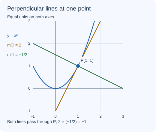
The point is (1,1) and y′=2x gives m=2. The tangent is \(y-1=2(x-1)\), or y=2x−1. The normal is \(y-1=-\tfrac12(x-1)\), or y=−x/2+3/2.
Example 2
Find the tangent and normal to y=x²+3 at x=0.
Show the reasoning
The point is (0,3), with gradient zero. The tangent is y=3 and the normal is x=0. The latter is a vertical line, not y=0.
Example 3
Find every point on y=x³−x whose tangent is parallel to y=2x+5.
Show the reasoning
Set 3x²−1=2, obtaining x=±1. Both ordinates are zero, so the points are (−1,0) and (1,0). Their tangents are y=2x+2 and y=2x−2 respectively.
Use derivative signs, classify stationary points and compare candidates for an absolute extremum.
Notes
Before you start: factor derivatives, solve inequalities and read signs on intervals.
Where f′>0 throughout an interval, f is strictly increasing; where f′<0, it is strictly decreasing. At a differentiable stationary point f′=0. A zero derivative alone does not establish a maximum or minimum: inspect the behaviour around the point.
A change in f′ from positive to negative gives a local maximum.
A change from negative to positive gives a local minimum.
No sign change may give a stationary point that is neither; investigate the curve.
If f′(a)=0 and f″(a)>0, the second derivative test gives a local minimum; f″(a)<0 gives a local maximum. If f″(a)=0, the test is inconclusive. A stationary point of inflection has a horizontal tangent and a change of concavity. Derivative signs or the actual function can resolve an inconclusive test.
A strictly increasing function can have an isolated zero derivative, as x³ does at zero. Do not split a monotonic interval merely because a derivative touches zero without changing sign.
A local extremum concerns nearby inputs. An absolute extremum concerns the entire stated domain. On a closed bounded interval, compare all interior stationary points, any interior points where a derivative fails, and the endpoints of a continuous function. On an open or unbounded domain, an endpoint or limiting value may not be attained.
Recall later
f′(a)=f″(a)=0 means “test inconclusive”, not “definitely an inflection”. Further reasoning is essential.
Common mistakes
Assuming every stationary point is a turning point.
Treating f″=0 as a conclusive classification.
Ignoring endpoints or reporting a local extremum as an absolute one without comparison.
Three worked examples
Example 1
Find the stationary points and monotonic intervals of f(x)=x³−3x.
Show the reasoning
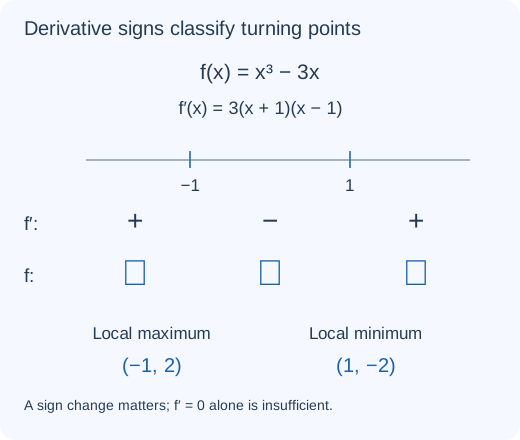
\(f^{\prime}=3(x-1)(x+1)\) is positive for x<−1 and x>1, negative for −1<x<1. The local maximum is (−1,2) and local minimum (1,−2), using the sign changes.
Example 2
Classify the stationary point of f(x)=x³.
Show the reasoning
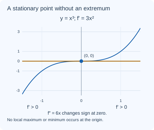
f′=3x² vanishes only at zero and is positive on both sides. Thus zero is not a maximum or minimum. Since f″=6x changes from negative to positive, (0,0) is a stationary point of inflection. The function is strictly increasing on the real line.
Example 3
Find the absolute maximum and minimum of f(x)=x²−4x+7 on 0≤x≤5.
Show the reasoning
f′=2x−4 gives the interior candidate x=2. Compare f(0)=7, f(2)=3 and f(5)=12. The absolute minimum is 3 at x=2; the absolute maximum is 12 at the included endpoint x=5.
Relate changing quantities through a derivative, keeping signs, units and approximation status.
Notes
Before you start: differentiate powers, use geometric formulas and convert units consistently.
If y=f(x) and x changes smoothly with time t, the chain rule gives
\[\frac{dy}{dt}=\frac{dy}{dx}\frac{dx}{dt}.\]
Evaluate the geometric derivative at the specified instant. A negative rate means a quantity is decreasing; it is not an instruction to discard a solution. If a volume has units cm³ and time has units s, its rate has units cm³/s, while a radius rate has units cm/s.
For a small change Δx, the linear estimate is \(\Delta y\approx f^{\prime}(x)\Delta x\). Use the derivative at the initial x. The exact change is f(x+Δx)−f(x); the two need not agree. Similarly, over a short time step, \(x(t+\Delta t)\approx x(t)+\dot x(t)\Delta t\). This is a local approximation, not permission to assume the rate stays constant indefinitely.
Recall later
If y=x², then Δy=2xΔx+(Δx)² exactly. The first-order estimate omits (Δx)².
Common mistakes
Confusing a geometric derivative with a time derivative.
Dropping a negative rate or using inconsistent length/volume units.
Writing an approximate small-increment relation as an exact finite change.
Three worked examples
Example 1
A sphere has V=4πr³/3. At r=2 cm, dr/dt=0.1 cm/s. Find dV/dt.
Show the reasoning
\(dV/dr=4\pi r^2\), so \(dV/dt=4\pi(2^2)(0.1)=1.6\pi\) cm³/s. Both the sign and the volume-per-time units are retained.
Example 2
An area y=3x² cm² depends on a length x cm. At x=5, dx/dt=−0.4 cm/s. Find dy/dt.
Show the reasoning
\(dy/dx=6x\), so \(dy/dt=6(5)(-0.4)=-12\) cm²/s. The area is decreasing at 12 cm²/s.
Example 3
Use differentiation to estimate the change in x² when x increases from 4 to 4.03; compare with the exact change.
Show the reasoning
Δx=0.03 and f′(4)=8, so Δy≈8(0.03)=0.24. The exact change is 4.03²−4²=0.2409. The linear estimate is low by 0.0009, the omitted square (0.03)².
Build a one-variable model, reject inadmissible stationary values and justify a global optimum.
Notes
Before you start: eliminate a variable from a constraint, differentiate, and interpret derivative signs.
Define the variables and state a feasible domain from the geometry or context.
Use the constraint to write the objective as a function of one variable.
Find stationary candidates and retain only those inside the feasible domain.
Classify candidates, compare appropriate boundary values or limits, and justify the optimum on the whole domain.
Give the requested dimensions or quantity with units, retaining exact values before rounding.
A negative second derivative at a stationary point proves a local maximum; it does not by itself prove a global maximum on an arbitrary domain. A complete derivative-sign argument, a suitable comparison with endpoints/limits, or an algebraic bound can establish the global result.
Geometric dimensions are usually positive. A root that gives a negative side, a zero-volume object or a dimension beyond the sheet is not admissible. On an open domain, boundary limits help compare values without pretending the boundary objects are feasible.
Recall later
For A=x(12−x), \(A=36-(x-6)^2\le36\). Equality occurs at the feasible value x=6, so the bound proves the global maximum directly.
Common mistakes
Solving the stationary equation without stating or checking a feasible domain.
Using only a local second-derivative test to claim a global optimum.
Giving an optimal input but omitting the requested output, other dimension or units.
Three worked examples
Example 1
A rectangle has perimeter 24 cm. Find its greatest area and dimensions.
Show the reasoning
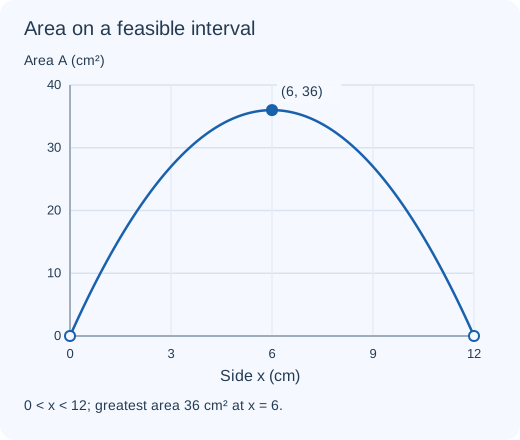
If the sides are x and y, x+y=12, so A=x(12−x), with 0<x<12. A′=12−2x vanishes at x=6. It is positive before 6 and negative afterwards, giving the global maximum 36 cm² at a 6 cm by 6 cm square.
Example 2
Find the least value of f(x)=x+9/x for x>0.
Show the reasoning
\(f^{\prime}=1-9/x^2=(x-3)(x+3)/x^2\). The only positive stationary input is 3. The derivative is negative on (0,3) and positive on (3,∞), proving the global minimum f(3)=6. The negative root is outside the domain.
Example 3
An open-top cylinder has volume 8π cm³. Minimise the area of its base and curved surface.
Show the reasoning
With r>0, the height is h=8/r² and the area is \(A=\pi r^2+16\pi/r\). Its derivative is \(2\pi(r^3-8)/r^2\), negative for 0<r<2 and positive for r>2. Hence the global minimum occurs at r=2 cm, h=2 cm, with A=12π cm².