Past Exam Questions
← Back9709 P61 - Jun 2014 - Q7
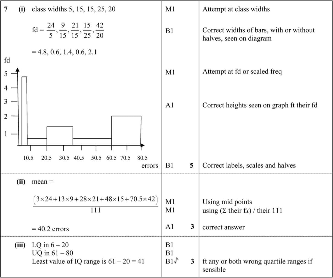
A typing test is taken by 111 people. The numbers of typing errors they make in the test are summarised in the table below.
| Number of typing errors | 1–5 | 6–20 | 21–35 | 36–60 | 61–80 |
|---|---|---|---|---|---|
| Frequency | 24 | 9 | 21 | 15 | 42 |
- Draw a histogram on graph paper to represent this information.
- Calculate an estimate of the mean number of typing errors for these 111 people.
- State which class contains the lower quartile and which class contains the upper quartile. Hence find the least possible value of the interquartile range.
9709 P63 - Nov 2013 - Q1
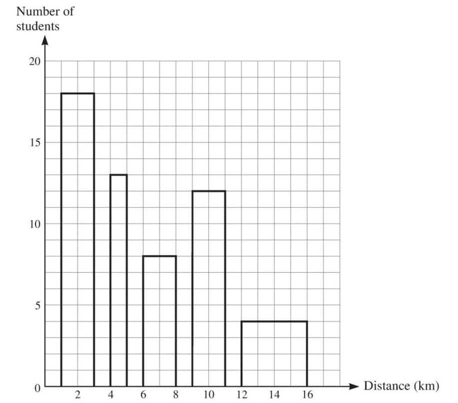
The distance of a student’s home from college, correct to the nearest kilometre, was recorded for each of 55 students. The distances are summarised in the following table.
| Distance from college (km) | 1–3 | 4–5 | 6–8 | 9–11 | 12–16 |
|---|---|---|---|---|---|
| Number of students | 18 | 13 | 8 | 12 | 4 |
Dominic is asked to draw a histogram to illustrate the data. Dominic’s diagram is shown below.
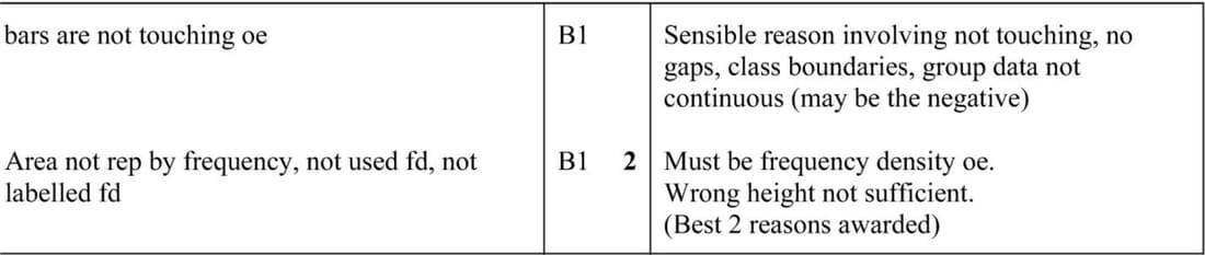
Give two reasons why this is not a correct histogram.
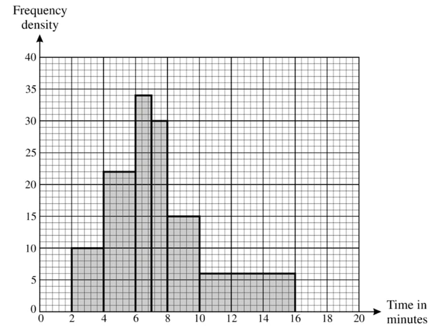
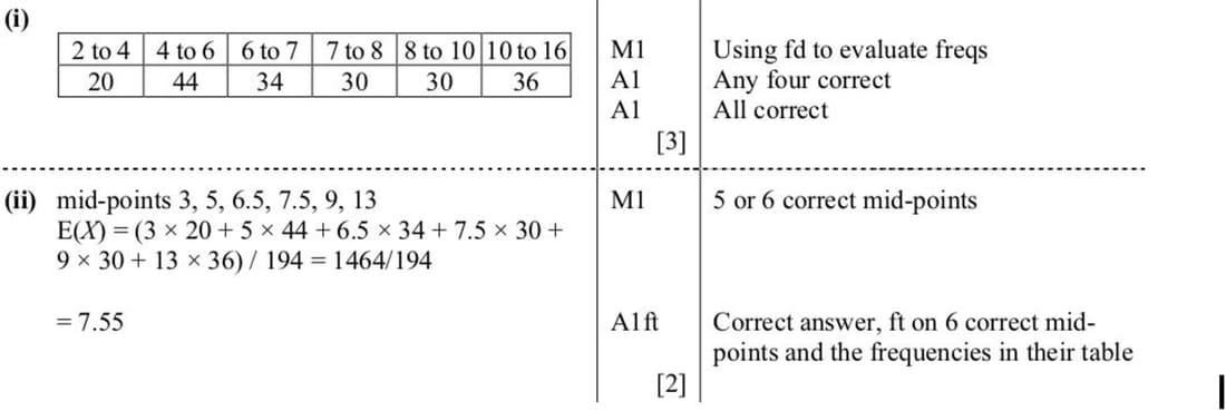
9709 P62 - Nov 2013 - Q4
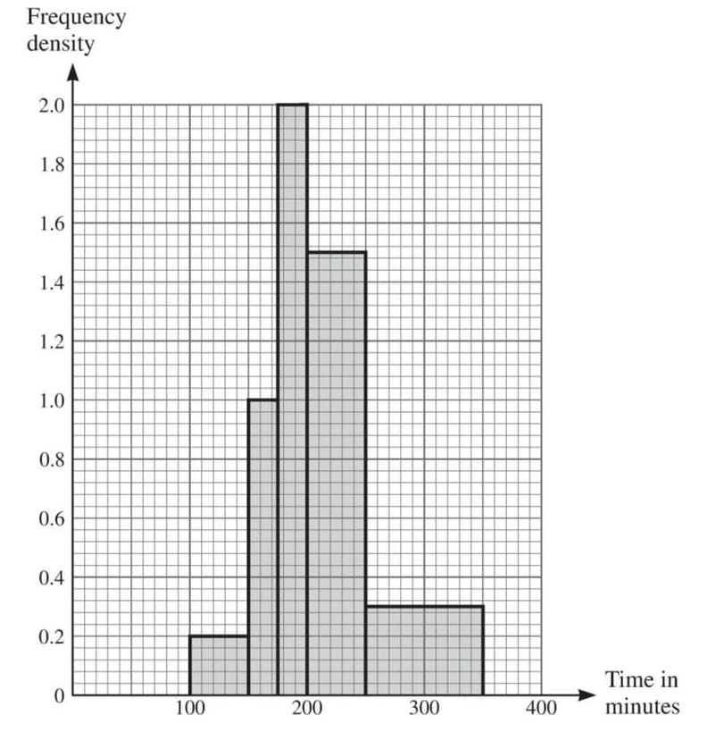
The following histogram summarises the times, in minutes, taken by 190 people to complete a race.
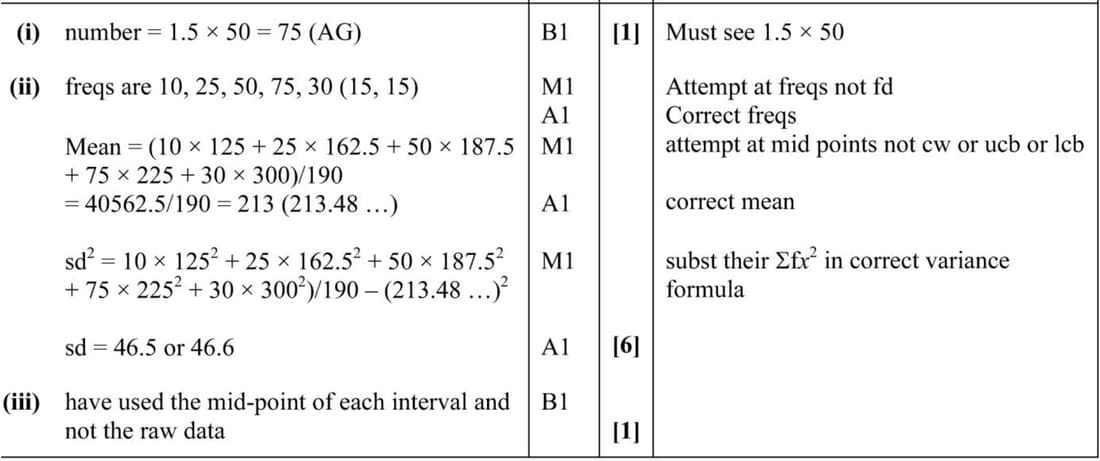
(i) Show that 75 people took between 200 and 250 minutes to complete the race.
(ii) Calculate estimates of the mean and standard deviation of the times of the 190 people.
(iii) Explain why your answers to part (ii) are estimates.
9709 P63 - Nov 2012 - Q4
In a survey, the percentage of meat in a certain type of take-away meal was found. The results, to the nearest integer, for 193 take-away meals are summarised in the table.
| Percentage of meat | 1–5 | 6–10 | 11–20 | 21–30 | 31–50 |
|---|---|---|---|---|---|
| Frequency | 59 | 67 | 38 | 18 | 11 |
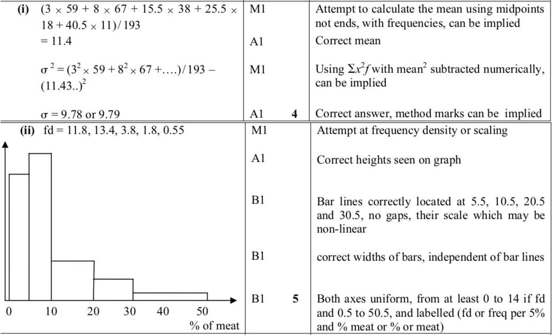
(i) Calculate estimates of the mean and standard deviation of the percentage of meat in these take-away meals.
(ii) Draw, on graph paper, a histogram to illustrate the information in the table.
9709 P62 - Nov 2012 - Q3
The table summarises the times that 112 people took to travel to work on a particular day.
| Time (minutes) | 0 < t ≤ 10 | 10 < t ≤ 15 | 15 < t ≤ 20 | 20 < t ≤ 25 | 25 < t ≤ 40 | 40 < t ≤ 60 |
|---|---|---|---|---|---|---|
| Frequency | 19 | 12 | 28 | 22 | 18 | 13 |
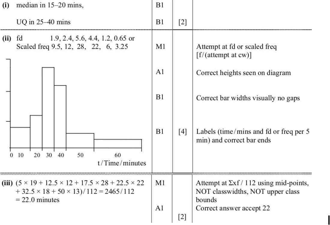
- State which time interval in the table contains the median and which time interval contains the upper quartile.
- On graph paper, draw a histogram to represent the data.
- Calculate an estimate of the mean time to travel to work.
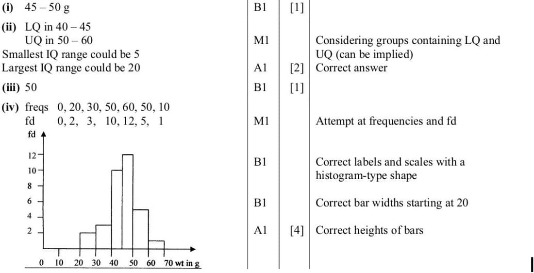
9709 P62 - Nov 2011 - Q4
The weights of 220 sausages are summarised in the following table.
| Weight (grams) | <20 | <30 | <40 | <45 | <50 | <60 | <70 |
|---|---|---|---|---|---|---|---|
| Cumulative frequency | 0 | 20 | 50 | 100 | 160 | 210 | 220 |
- State which interval the median weight lies in.
- Find the smallest possible value and the largest possible value for the interquartile range.
- State how many sausages weighed between 50 g and 60 g.
- On graph paper, draw a histogram to represent the weights of the sausages.
9709 P63 - Nov 2010 - Q5
The following histogram illustrates the distribution of times, in minutes, that some students spent taking a shower.
(i) Copy and complete the following frequency table for the data.
| Time \( t \) (minutes) | \( 2 < t \le 4 \) | \( 4 < t \le 6 \) | \( 6 < t \le 7 \) | \( 7 < t \le 8 \) | \( 8 < t \le 10 \) | \( 10 < t \le 16 \) |
|---|---|---|---|---|---|---|
| Frequency |
(ii) Calculate an estimate of the mean time to take a shower.
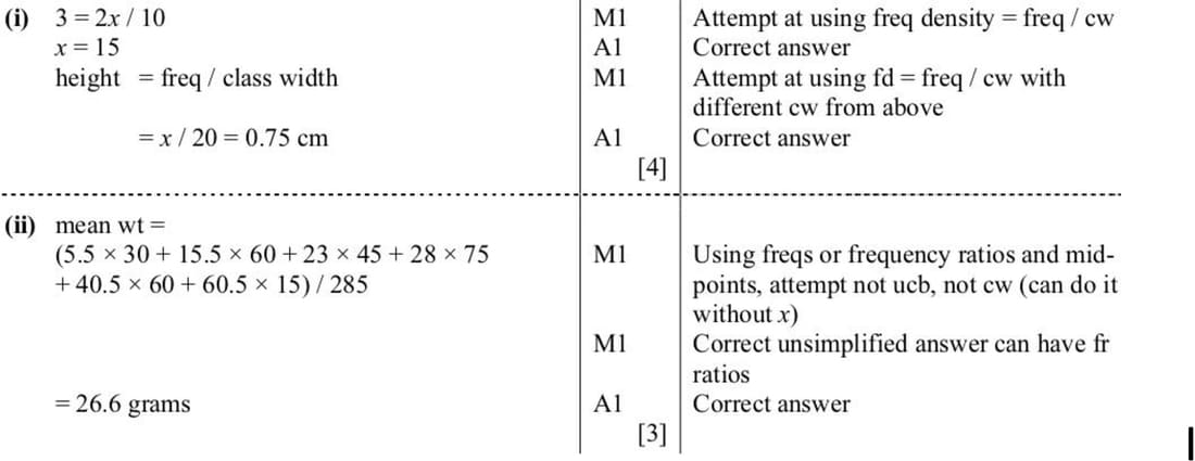
9709 P61 - Nov 2010 - Q4
The weights in grams of a number of stones, measured correct to the nearest gram, are represented in the following table.
| Weight (grams) | 1–10 | 11–20 | 21–25 | 26–30 | 31–50 | 51–70 |
|---|---|---|---|---|---|---|
| Frequency | 2x | 4x | 3x | 5x | 4x | x |
A histogram is drawn with a scale of 1 cm to 1 unit on the vertical axis, which represents frequency density. The 1–10 rectangle has height 3 cm.
(i) Calculate the value of \( x \) and the height of the 51–70 rectangle.
(ii) Calculate an estimate of the mean weight of the stones.
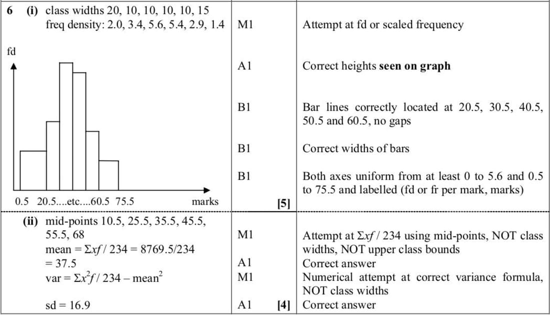
9709 P62 - Nov 2009 - Q6
The following table gives the marks, out of 75, in a pure mathematics examination taken by 234 students.
| Marks | 1–20 | 21–30 | 31–40 | 41–50 | 51–60 | 61–75 |
|---|---|---|---|---|---|---|
| Frequency | 40 | 34 | 56 | 54 | 29 | 21 |
(i) Draw a histogram on graph paper to represent these results.
(ii) Calculate estimates of the mean mark and the standard deviation.
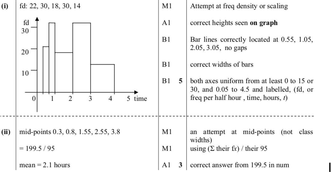
9709 P6 - Jun 2008 - Q5
As part of a data collection exercise, members of a certain school year group were asked how long they spent on their Mathematics homework during one particular week. The times are given to the nearest 0.1 hour. The results are displayed in the following table.
| Time spent \( t \) (hours) | \( 0.1 \le t \le 0.5 \) | \( 0.6 \le t \le 1.0 \) | \( 1.1 \le t \le 2.0 \) | \( 2.1 \le t \le 3.0 \) | \( 3.1 \le t \le 4.5 \) |
|---|---|---|---|---|---|
| Frequency | 11 | 15 | 18 | 30 | 21 |
(i) Draw, on graph paper, a histogram to illustrate this information.
(ii) Calculate an estimate of the mean time spent on their Mathematics homework by members of this year group.
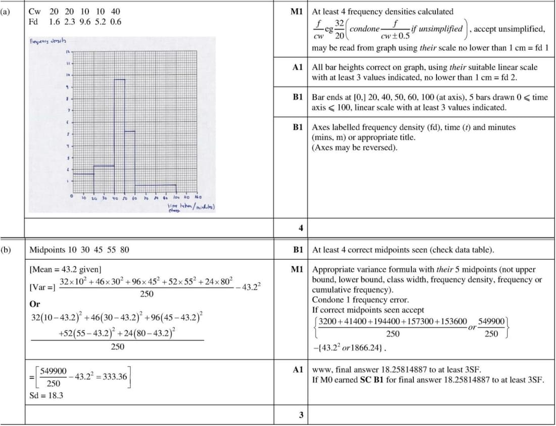
9709 P52 - Nov 2022 - Q4
The times taken, in minutes, to complete a word processing task by 250 employees at a particular company are summarised in the table.
| Time taken \( t \) (minutes) | \( 0 \le t \lt 20 \) | \( 20 \le t \lt 40 \) | \( 40 \le t \lt 50 \) | \( 50 \le t \lt 60 \) | \( 60 \le t \lt 100 \) |
|---|---|---|---|---|---|
| Frequency | 32 | 46 | 96 | 52 | 24 |
(a) Draw a histogram to represent this information.
From the data, the estimate of the mean time taken by these 250 employees is \( 43.2 \) minutes.
(b) Calculate an estimate for the standard deviation of these times.
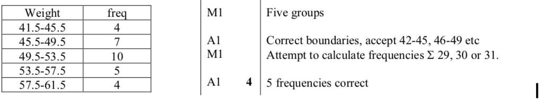
9709 P6 - Nov 2006 - Q1
The weights of 30 children in a class, to the nearest kilogram, were as follows:
50, 45, 61, 53, 55, 47, 52, 49, 46, 51, 60, 52, 54, 47, 57, 59, 42, 46, 51, 53, 56, 48, 50, 51, 44, 52, 49, 58, 55, 45
Construct a grouped frequency table for these data such that there are five equal class intervals with the first class having a lower boundary of 41.5 kg and the fifth class having an upper boundary of 61.5 kg.
9709 P6 - Jun 2006 - Q5
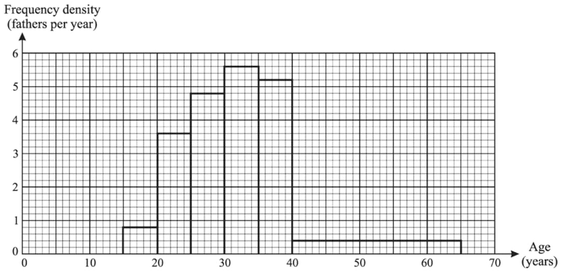
Each father in a random sample of fathers was asked how old he was when his first child was born. The following histogram represents the information.
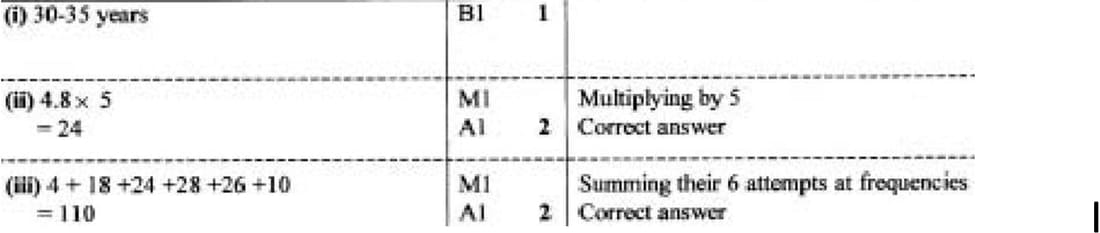
- What is the modal age group?
- How many fathers were between 25 and 30 years old when their first child was born?
- How many fathers were in the sample?
9709 P6 - Nov 2004 - Q2
The lengths of cars travelling on a car ferry are noted. The data are summarised in the following table.
| Length of car \( x \) (metres) | \( 2.80 \le x < 3.00 \) | \( 3.00 \le x < 3.10 \) | \( 3.10 \le x < 3.20 \) | \( 3.20 \le x < 3.40 \) |
|---|---|---|---|---|
| Frequency | 17 | 24 | 19 | 8 |
| Frequency density | 85 | 240 | 190 | \( a \) |
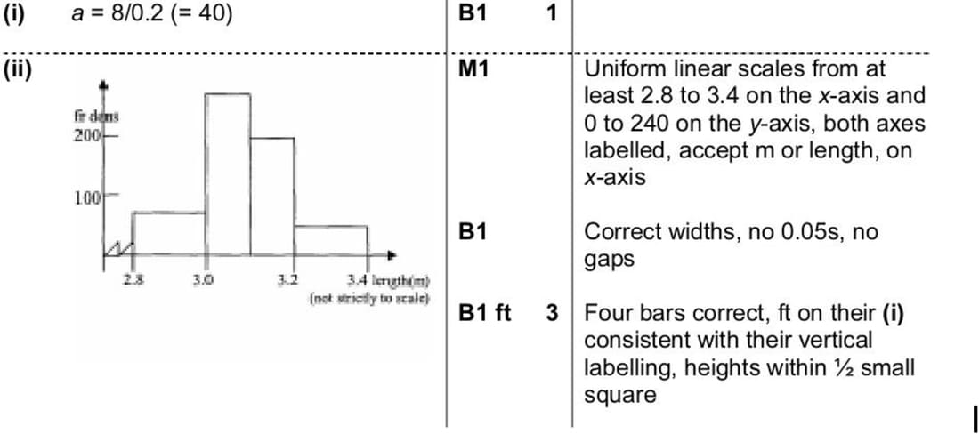
(i) Find the value of \( a \).
(ii) Draw a histogram on graph paper to represent the data.
9709 P6 - Nov 2003 - Q2
The floor areas, \( x \) m\(^2\), of 20 factories are as follows:
150, 350, 450, 578, 595, 644, 722, 798, 802, 904, 1000, 1330, 1533, 1561, 1778, 1960, 2167, 2330, 2433, 3231
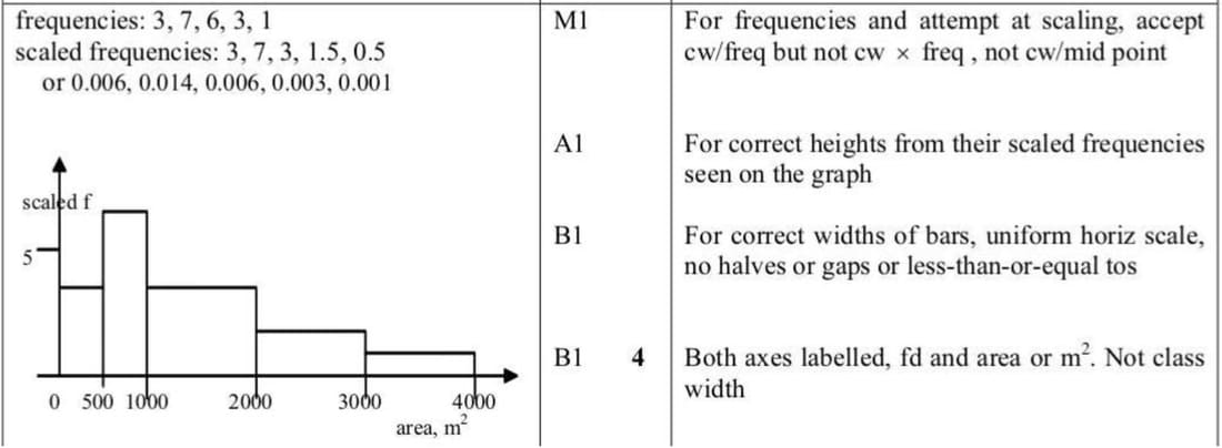
Represent these data by a histogram on graph paper, using intervals:
- \( 0 \le x < 500 \)
- \( 500 \le x < 1000 \)
- \( 1000 \le x < 2000 \)
- \( 2000 \le x < 3000 \)
- \( 3000 \le x < 4000 \)
9709 P6 - Jun 2003 - Q7
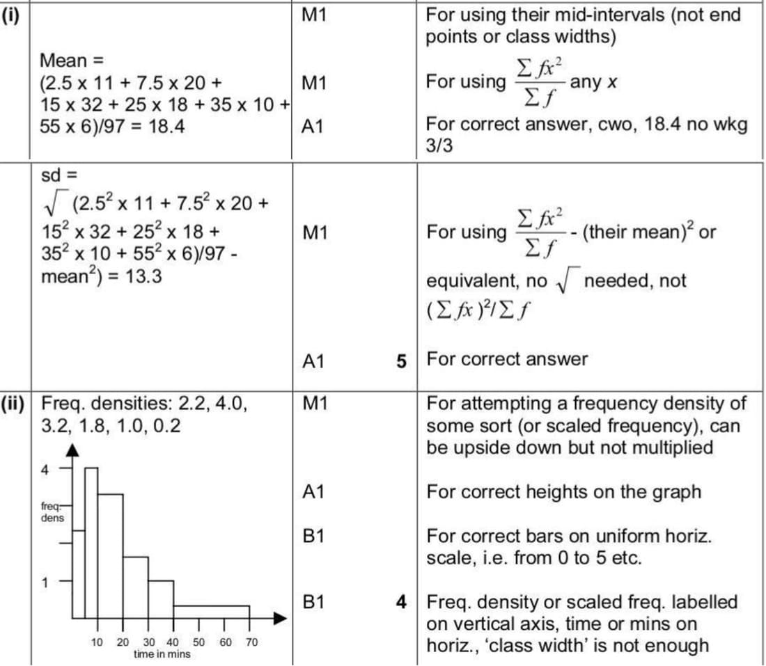
A random sample of 97 people who own mobile phones was used to collect data on the amount of time they spent per day on their phones. The results are displayed in the table below.
| Time spent per day \( t \) (minutes) | \( 0 \le t < 5 \) | \( 5 \le t < 10 \) | \( 10 \le t < 20 \) | \( 20 \le t < 30 \) | \( 30 \le t < 40 \) | \( 40 \le t < 70 \) |
|---|---|---|---|---|---|---|
| Frequency (people) | 11 | 20 | 32 | 18 | 10 | 6 |
(i) Calculate estimates of the mean and standard deviation of the time spent per day on these mobile phones.
(ii) On graph paper, draw a fully labelled histogram to represent the data.
9709 P51 - Jun 2022 - Q3
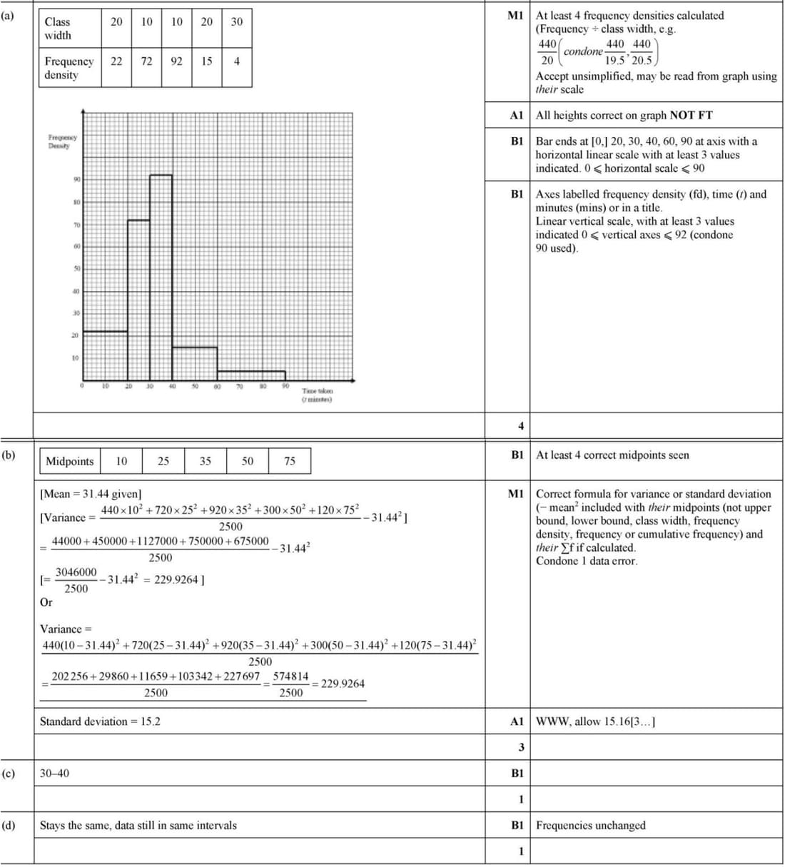
The times taken to travel to college by 2500 students are summarised in the table.
| Time taken \( t \) (minutes) | \( 0 \le t < 20 \) | \( 20 \le t < 30 \) | \( 30 \le t < 40 \) | \( 40 \le t < 60 \) | \( 60 \le t < 90 \) |
|---|---|---|---|---|---|
| Frequency | 440 | 720 | 920 | 300 | 120 |
(a) Draw a histogram to represent this information.
From the data, the estimate of the mean value of \( t \) is \( 31.44 \).
(b) Calculate an estimate of the standard deviation of the times taken to travel to college.
(c) In which class interval does the upper quartile lie?
It was later discovered that the times taken to travel to college by two students were incorrectly recorded. One student’s time was recorded as \( 15 \) instead of \( 5 \) and the other’s time was recorded as \( 65 \) instead of \( 75 \).
(d) Without doing any further calculations, state with a reason whether the estimate of the standard deviation in part (b) would be increased, decreased or stay the same.
9709 P52 - Mar 2022 - Q3
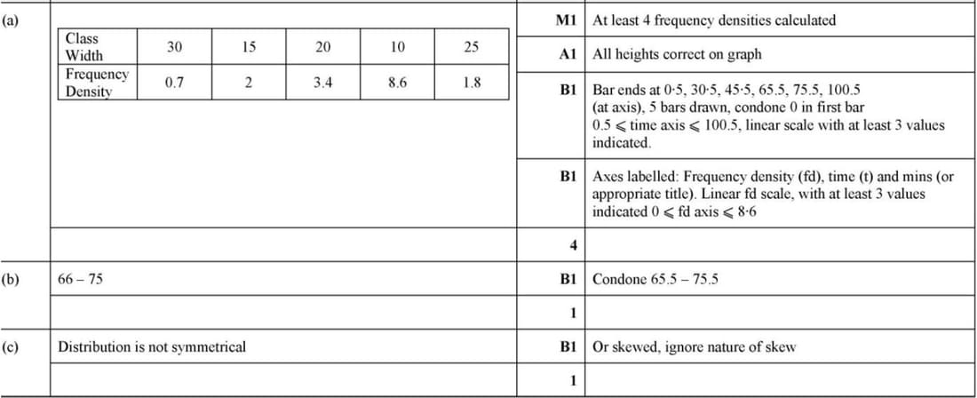
At a summer camp an arithmetic test is taken by 250 children. The times taken, to the nearest minute, to complete the test were recorded. The results are summarised in the table.
| Time taken (minutes) | 1–30 | 31–45 | 46–65 | 66–75 | 76–100 |
|---|---|---|---|---|---|
| Frequency | 21 | 30 | 68 | 86 | 45 |
(a) Draw a histogram to represent this information.
(b) State which class interval contains the median.
(c) Given that an estimate of the mean time is 61.05 minutes, state what feature of the distribution accounts for the median and the mean being different.
9709 P53 - Nov 2021 - Q3
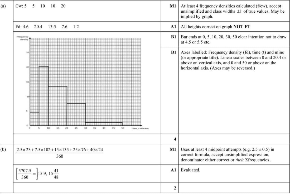
The times taken, in minutes, by 360 employees at a large company to travel from home to work are summarised in the following table.
| Time \( t \) (minutes) | \( 0 \le t < 5 \) | \( 5 \le t < 10 \) | \( 10 \le t < 20 \) | \( 20 \le t < 30 \) | \( 30 \le t < 50 \) |
|---|---|---|---|---|---|
| Frequency | 23 | 102 | 135 | 76 | 24 |
(a) Draw a histogram to represent this information.
(b) Calculate an estimate of the mean time taken by an employee to travel to work.
9709 P51 - Jun 2021 - Q5
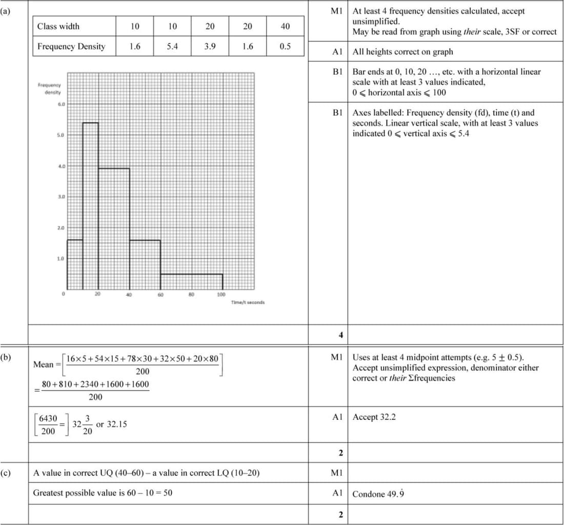
The times taken by 200 players to solve a computer puzzle are summarised in the following table.
| Time \( t \) (seconds) | \( 0 \le t < 10 \) | \( 10 \le t < 20 \) | \( 20 \le t < 40 \) | \( 40 \le t < 60 \) | \( 60 \le t < 100 \) |
|---|---|---|---|---|---|
| Number of players | 16 | 54 | 78 | 32 | 20 |
- Draw a histogram to represent this information.
- Calculate an estimate of the mean time taken by these 200 players.
- Find the greatest possible value of the interquartile range of these times.