Use area and integration to find probabilities, averages and percentiles for measurements.
By the end of this lesson
- Check and normalise a probability density function.
- Calculate interval probabilities and percentiles.
- Find the mean, variance and standard deviation by integration.
- Handle a simple density with an infinite support.
Before you begin: Integrate powers of x using definite integrals.; Rearrange equations and work with exact fractions.; Recall expectation and variance for a discrete random variable..
1. Probability is an area
A continuous model describes a measurement that can take any value in an interval, such as time or length. Its probability density function, written $f(x)$, shows how probability is distributed. The support is the set of possible values in the model; the density is zero outside it.
Key formula
Conditions for a valid density
Check nonnegativity throughout the support as well as total area. Both conditions are necessary.
A density height is not a probability. For example, a rectangle of height $2$ and width $0.5$ has area $1$, so it can define a valid density. If $X$ is measured in seconds, its density has units of inverse seconds; multiplying height by width produces a dimensionless probability.
Key formula
Probability between two values
Integrate only where the interval meets the support. For a continuous variable, $\operatorname{P}(X=a)=0$, so including a single endpoint does not change the answer.
2. Find the constant before the probability
If a density contains an unknown constant, use total probability $1$ to find it. Then substitute the constant into the density before calculating other areas. Sketching the support first helps you choose sensible integration limits.
Worked example
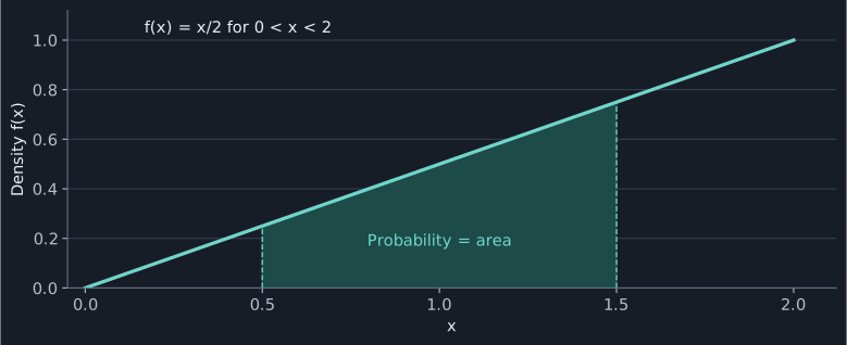
A rising density
The density is $f(x)=kx$ for $0<x<2$ and zero elsewhere. Find $k$ and $\operatorname{P}(0.5<X<1.5)$.
Set the area over the entire support equal to one.
\[\int_0^2 kx\,\mathrm{d}x=k\left[\frac{x^2}{2}\right]_0^2=2k=1\]Hence $k=\frac12$. The resulting density is nonnegative throughout its support.
Integrate this density over the requested interval.
\[\operatorname{P}(0.5<X<1.5)=\left[\frac{x^2}{4}\right]_{0.5}^{1.5}=\frac{2.25-0.25}{4}=\frac12\]

3. Mean and variance of a continuous model
Expectation uses the same weighting idea as a discrete distribution, with integration replacing summation. The mean is the long-run average of observations from the model. First calculate the two moments below, and then subtract the square of the mean.
Key formula
Continuous moments
Both integrals are over the whole support, and the moments must exist.
Key formula
Variance and standard deviation
Variance has squared measurement units. Standard deviation has the same units as $X$.
Worked example
Moments of the rising density
For $f(x)=x/2$ on $0<x<2$, find the mean, variance and standard deviation.
Multiply the density by x for the first moment.
\[\operatorname{E}(X)=\int_0^2\frac{x^2}{2}\,\mathrm{d}x=\left[\frac{x^3}{6}\right]_0^2=\frac43\]Multiply the density by x squared for the second moment.
\[\operatorname{E}(X^2)=\int_0^2\frac{x^3}{2}\,\mathrm{d}x=\left[\frac{x^4}{8}\right]_0^2=2\]Subtract using exact fractions.
\[\operatorname{Var}(X)=2-\left(\frac43\right)^2=\frac29,\qquad \operatorname{SD}(X)=\frac{\sqrt2}{3}\]
4. Medians and percentiles divide the area
The median $m$ has half the probability to its left. More generally, a percentile is a value below which a specified proportion of the distribution lies. These are statements about area, so the median need not be halfway between the support endpoints.
Key formula
Find a percentile
For a median use $p=0.5$; for the upper quartile use $p=0.75$. Select a solution within the support.
For $f(x)=x/2$ on $0<x<2$, the area to the left of $q$ is $q^2/4$. The median solves $m^2/4=1/2$, giving $m=\sqrt2$. The upper quartile solves $q^2/4=3/4$, giving $q=\sqrt3$. Both exceed $1$, which fits the greater density towards the right.
5. When the support continues indefinitely
An infinite integration limit means a limit of finite integrals. Replace infinity by a number $b$, integrate, and then let $b$ increase without bound. Total probability must converge to $1$. A valid density does not automatically have a finite mean or variance: those integrals need checking separately.
Worked example
An infinite tail
Let $f(x)=3/x^4$ for $x\geq1$ and zero elsewhere. Check the density and find $\operatorname{P}(X>2)$, the mean and the variance.
The density is nonnegative for $x\geq1$. Its total area is
\[\lim_{b\to\infty}\int_1^b3x^{-4}\,\mathrm{d}x=\lim_{b\to\infty}(1-b^{-3})=1\]For the tail probability, change the lower limit to two.
\[\operatorname{P}(X>2)=\lim_{b\to\infty}\left(\frac18-b^{-3}\right)=\frac18\]Both moment integrals converge.
\[\operatorname{E}(X)=\int_1^\infty3x^{-3}\,\mathrm{d}x=\frac32,\qquad \operatorname{E}(X^2)=\int_1^\infty3x^{-2}\,\mathrm{d}x=3\]Use the variance identity.
\[\operatorname{Var}(X)=3-\left(\frac32\right)^2=\frac34\]
6. A reliable calculation routine
- Identify the support and set the density to zero elsewhere.
- Normalise if necessary, then select the integral that matches the question.
- Use exact fractions until the final numerical answer.
- Check probabilities lie between zero and one, percentiles lie in the support, and variances are nonnegative.
Practice
Try each question before opening its worked solution.
Question 1
Let $f(x)=2x$ for $0<x<1$, zero elsewhere. Find (a) $\operatorname{P}(X>0.5)$ and (b) the median.
Show worked solution
Integrate from the threshold to the upper support limit.
\[\operatorname{P}(X>0.5)=\int_{0.5}^1 2x\,\mathrm{d}x=[x^2]_{0.5}^1=\frac34\]The median has area one half to its left.
\[\int_0^m2x\,\mathrm{d}x=m^2=\frac12\]
Question 2
A density is $f(x)=k(1+x)$ on $0<x<1$, zero elsewhere. Find $k$, the mean and the variance.
Show worked solution
Normalise over the support.
\[k\int_0^1(1+x)\,\mathrm{d}x=\frac{3k}{2}=1\quad\Rightarrow\quad k=\frac23\]Calculate both moments.
\[\operatorname{E}(X)=\frac23\left(\frac12+\frac13\right)=\frac59,\qquad \operatorname{E}(X^2)=\frac23\left(\frac13+\frac14\right)=\frac7{18}\]Subtract the squared mean.
\[\operatorname{Var}(X)=\frac7{18}-\frac{25}{81}=\frac{13}{162}\]
Question 3
A density equals $4$ on $1<x<1.25$ and zero elsewhere. Explain why it is valid, then find $\operatorname{P}(1.1<X<1.2)$ and the median.
Show worked solution
The density is nonnegative and its total area is $4(1.25-1)=1$.
The requested probability is the rectangle area $4(1.2-1.1)=0.4$.
For the median, $4(m-1)=0.5$, so $m=1.125$.
Question 4
Let $f(x)=3x^2$ for $0<x<1$, zero elsewhere. Find the mean, variance and upper quartile.
Show worked solution
Calculate the moments over the support.
\[\operatorname{E}(X)=\int_0^1 3x^3\,\mathrm{d}x=\frac34,\qquad \operatorname{E}(X^2)=\int_0^1 3x^4\,\mathrm{d}x=\frac35\]Find the variance.
\[\operatorname{Var}(X)=\frac35-\frac9{16}=\frac3{80}\]Set the area to the left of the upper quartile equal to 0.75.
\[\int_0^q3x^2\,\mathrm{d}x=q^3=\frac34\]
Apply the same area interpretation to an important continuous model, then use standardisation to calculate its probabilities.