Use standardisation, areas and percentiles, then approximate suitable binomial probabilities.
By the end of this lesson
- Standardise a normal variable and calculate tail or interval probabilities.
- Find percentiles and recover model parameters from probability information.
- Choose a suitable normal approximation to a binomial distribution.
- Apply the correct continuity correction.
Before you begin: Mean, variance and standard deviation; Continuous probability as area; Binomial mean and variance; Solving simultaneous linear equations.
1. Reading a normal model
A normal distribution is continuous, symmetric and bell-shaped. Its mean $\mu$ gives the centre, and its standard deviation $\sigma$ controls the spread. Total area under its density curve is 1, with half on each side of the mean. A normal model can describe measurements, but the modelling assumption must be justified by the context.
Key formula
Normal notation
The second parameter is the variance. Take $\sigma>0$ and use $\sigma$, not $\sigma^2$, when standardising.
For $X\sim\mathrm N(50,64)$, the mean is 50 and the standard deviation is $\sqrt{64}=8$. The mean has the units of $X$, while variance has squared units. Since the distribution is continuous, $P(X=c)=0$ for any single value $c$; changing an endpoint from $<$ to $\le$ does not change a normal probability.
2. Convert to a standard normal variable
Standardisation expresses a measurement as a number of standard deviations above or below the mean. Subtracting the mean centres the distribution at zero; dividing by the standard deviation gives variance 1. A negative standardised value lies below the mean.
Key formula
Standardisation
Use when $X$ is normally distributed. Write $\Phi(z)=P(Z\le z)$ for the standard normal cumulative probability.
| Area needed | Expression |
|---|---|
| Left of $z$ | $\Phi(z)$ |
| Right of $z$ | $1-\Phi(z)$ |
| Between $a$ and $b$ | $\Phi(b)-\Phi(a)$ |
| Left of $-z$ | $\Phi(-z)=1-\Phi(z)$ |
Check what your table provides: some tables report a left cumulative area, while others give the area between zero and a positive value. For a left cumulative table, $\Phi(1.25)\approx0.8944$. Sketch and shade the required region before reading a value or using a calculator.
3. Tails and intervals

Worked example
Worked example 1: two areas under one model
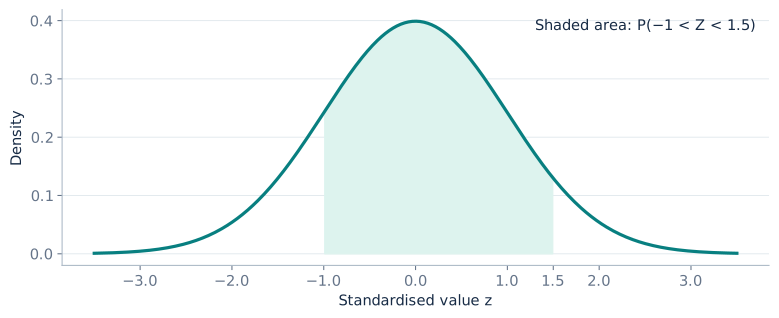
$X\sim\mathrm N(50,64)$. Find (a) $P(X>60)$ and (b) $P(42<X<62)$.
The standard deviation is $8$. For part (a), standardise the boundary and use the upper tail.
\[P(X>60)=P\left(Z>\frac{60-50}{8}\right)=1-\Phi(1.25)\]Evaluate the right-hand area.
\[P(X>60)=0.1056498\ldots\]For part (b), standardise both endpoints.
\[\frac{42-50}{8}=-1,\qquad\frac{62-50}{8}=1.5\]Subtract cumulative areas in the correct order.
\[P(42<X<62)=\Phi(1.5)-\Phi(-1)=0.7745375\ldots\]
4. Percentiles and unknown parameters
A percentile reverses the probability calculation: the area is known and the boundary is unknown. If $P(X\le c)=a$, first find the standard normal value $z_a$ with $\Phi(z_a)=a$. Then undo standardisation. For an upper-tail probability $b$, use left area $a=1-b$.
Key formula
Inverse normal calculation
For a normal variable and a cumulative probability $0<a<1$.
For example, the 90th percentile uses $z_{0.90}\approx1.2816$, while an upper 5% cutoff uses $z_{0.95}\approx1.645$. If both $\mu$ and $\sigma$ are unknown, two distinct percentile statements produce two simultaneous equations.
Worked example
Worked example 2: recovering centre and spread
A normal variable has 10th percentile 40 and 90th percentile 60. Find its mean and standard deviation.
By symmetry, $z_{0.10}=-1.2815516\ldots$ and $z_{0.90}=1.2815516\ldots$.
\[40=\mu-1.2815516\sigma,\qquad60=\mu+1.2815516\sigma\]Add the equations to eliminate the standard deviation.
\[100=2\mu\quad\Longrightarrow\quad\mu=50\]Subtract the equations, using unrounded values in the calculation.
\[20=2(1.2815516)\sigma\quad\Longrightarrow\quad\sigma\approx7.80304\]
5. When a binomial normal approximation is useful
A binomial distribution can be approximated by a normal distribution when both expected successes and expected failures are sufficiently large. Common guidance is to check $np>5$ and $n(1-p)>5$. These conditions guide an approximation; they do not make the two distributions identical. A large $n$ alone is not enough if $p$ is extremely close to 0 or 1.
Key formula
Match the binomial moments
Use $Y$ as an approximation when both $np$ and $n(1-p)$ are sufficiently large. Apply continuity correction before standardising.
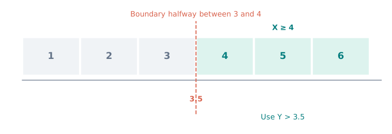
The binomial variable is integer-valued, whereas the normal variable is continuous. Represent each integer count by a unit-width interval centred on it. A continuity correction moves the probability boundary to the appropriate edge of this interval.
6. Continuity correction
| Binomial event | Normal approximation region |
|---|---|
| $X\le k$ | $Y<k+0.5$ |
| $X<k$ | $Y<k-0.5$ |
| $X\ge k$ | $Y>k-0.5$ |
| $X>k$ | $Y>k+0.5$ |
| $a\le X\le b$ | $a-0.5<Y<b+0.5$ |
Worked example
Worked example 3: a corrected upper tail
$X\sim\mathrm B(100,0.4)$. Use a normal approximation to estimate $P(X\ge48)$.
Check the conditions and match the mean and variance.
\[np=40,\quad n(1-p)=60,\quad Y\sim\mathrm N(40,24)\]Count 48 is included, so use the boundary halfway between 47 and 48.
\[P(X\ge48)\approx P(Y>47.5)\]Standardise using the square root of the variance.
\[P(Y>47.5)=1-\Phi\left(\frac{47.5-40}{\sqrt{24}}\right)\approx0.0629\]
For strict inequalities, identify the last or first included integer before correcting. For example, $X<8$ includes at most 7, so its upper boundary is $7.5$. Correcting directly to $8.5$ would include an unwanted integer.
7. Final checks before accepting an answer
- Have you identified $\sigma$ from the variance?
- Does your shaded region match the required tail or interval?
- For inverse calculations, does the percentile lie on the correct side of the mean?
- For a binomial approximation, have you checked both conditions and corrected before standardising?
Normal areas will reappear in sampling distributions, confidence intervals and hypothesis tests. Keeping the model, standardised boundary and area statement visible now makes those later methods much easier to follow.
Practice
Try each question before opening its worked solution.
Question 1
$Y\sim\mathrm N(60,100)$. Find (a) $P(Y>75)$ and (b) $P(45<Y<70)$.
Show worked solution
The standard deviation is $10$. Standardise each boundary.
\[P(Y>75)=1-\Phi(1.5)=0.0668072\ldots\]For the interval, subtract the two cumulative probabilities.
\[P(45<Y<70)=\Phi(1)-\Phi(-1.5)=0.7745375\ldots\]
Question 2
For $Y\sim\mathrm N(60,100)$, find (a) the 90th percentile and (b) the cutoff with 5% of values above it.
Show worked solution
Use the inverse formula with standard deviation 10.
\[c_{0.90}=60+1.2815516(10)=72.815516\ldots\]An upper 5% tail has left cumulative area 0.95.
\[c_{0.95}=60+1.6448536(10)=76.448536\ldots\]
Question 3
$X\sim\mathrm B(80,0.25)$. Justify a normal approximation and estimate (a) $P(X\le25)$ and (b) $P(16\le X\le24)$.
Show worked solution
Both expected counts exceed 5.
\[np=20,\quad n(1-p)=60,\quad Y\sim\mathrm N(20,15)\]Include count 25 using the boundary 25.5.
\[P(X\le25)\approx\Phi\left(\frac{5.5}{\sqrt{15}}\right)\approx0.922\]Include both integer endpoints with outward half-unit corrections.
\[P(16\le X\le24)\approx\Phi\left(\frac{4.5}{\sqrt{15}}\right)-\Phi\left(\frac{-4.5}{\sqrt{15}}\right)\approx0.755\]
Question 4
$T\sim\mathrm N(100,16)$. A student standardises 108 as $(108-100)/16=0.5$. Correct the calculation and find $P(T>108)$. Is continuity correction needed?
Show worked solution
The second parameter is variance, so divide by its square root.
\[z=\frac{108-100}{\sqrt{16}}=2\]Use the upper-tail probability.
\[P(T>108)=1-\Phi(2)=0.0227501\ldots\]The original variable is already continuous and normal. No continuity correction is needed.
Build another essential discrete model, this time for events counted in a fixed interval.