Calculate how long a sequence of independent trials waits for its first success.
By the end of this lesson
- Recognise a geometric experiment and define its trial count.
- Calculate first-success and tail probabilities.
- Use the mean to interpret or determine the success probability.
- Distinguish a waiting-time variable from a binomial success count.
Before you begin: Independent trials and complementary probabilities; Powers and simple probability products; The meaning of an expected value.
1. Count trials up to and including success
A geometric variable counts how many trials are needed to obtain the first success. The stopping point is random: the first trial may succeed, or many failures may occur first. Use the same definition of success on every trial. As with a binomial model, success can mean any outcome being studied, including a fault.
- Trials are independent.
- Every trial has success or failure as its two possible categories.
- The success probability $p$ is constant, with $0<p\le1$.
- Continue until the first success, including that successful trial in the count.
Key formula
Model and support
Cambridge counts trials including the first success. Write $q=1-p$ for the failure probability.
The smallest possible value is 1, because success on the first trial still uses one trial. There is no fixed largest possible value when $0<p<1$. Some sources define a geometric variable as the number of failures before success; that variable starts at 0. Always state your definition to avoid shifting every answer by one.
2. First success on a specified trial
The event $X=r$ requires exactly $r-1$ failures, followed by one success. This ordering is compulsory: an earlier success would stop the experiment. Independence allows the probabilities to be multiplied. No combinations factor is needed because there is only one permitted success-failure pattern.
Key formula
Geometric probability
For integer $r\ge1$, with independent trials and constant success probability $0<p\le1$.
Worked example
Worked example 1: first success on trial 4
An independent attempt succeeds with probability $0.3$. Attempts continue until success. Find the probability that the first success occurs on attempt 4.
Let $X$ count attempts including the successful attempt. Then $X\sim\mathrm{Geo}(0.3)$.
Trial 4 must be preceded by three failures: failure, failure, failure, success.
\[P(X=4)=(0.7)^3(0.3)\]Evaluate the product.
\[P(X=4)=0.1029\]
3. After, at least and within
Tail probabilities have a particularly simple form. If $X>r$, the first $r$ trials must all fail. There is no need to specify when success happens after them. If $X\ge r$, only the first $r-1$ trials must fail: success on trial $r$ is allowed.
Key formula
After r trials
Use integer $r\ge0$. “Within the first $r$ trials” means $X\le r$.
Key formula
At least r trials
Use integer $r\ge1$. Compare the included starting value carefully.
Worked example
Worked example 2: success within five attempts
Each independent attempt succeeds with probability $0.2$. Find the probability of (a) needing more than five attempts and (b) succeeding within five attempts.
Let $X\sim\mathrm{Geo}(0.2)$, so the failure probability is $q=0.8$.
More than five attempts requires five initial failures.
\[P(X>5)=(0.8)^5=0.32768\]Within five attempts is the complementary event.
\[P(X\le5)=1-(0.8)^5=0.67232\]
For an interval, subtract tails. First success from trial $a$ through trial $b$, inclusive, means waiting at least $a$ trials but not more than $b$. Thus $P(a\le X\le b)=q^{a-1}-q^b$ for integers $1\le a\le b$. Listing the endpoint trials before calculating helps prevent an off-by-one error.
4. Expected waiting time
The expected value describes the average number of trials over many repetitions of the whole waiting experiment. A smaller success probability gives a longer expected wait. This average is not a deadline, and success does not become more likely merely because several failures have occurred.
Key formula
Mean number of trials
For $X\sim\mathrm{Geo}(p)$ with $0<p\le1$, counting the successful trial.
Worked example
Worked example 3: recovering the probability
A repeated independent experiment has a geometric waiting time with mean 5 trials. Find the success probability and the probability of success within the first three trials.
Use the expected-value formula to recover the probability.
\[\frac1p=5\quad\Longrightarrow\quad p=0.2\]The failure probability is $0.8$. Within three trials is the complement of three failures.
\[P(X\le3)=1-(0.8)^3=1-0.512\]Evaluate and interpret the cumulative probability.
\[P(X\le3)=0.488\]
5. Shape and the effect of previous failures
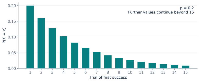
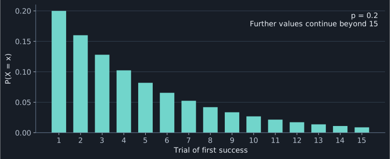
For $0<p<1$, each bar is $q$ times the preceding bar, so probabilities decrease as the trial number increases. Nevertheless, many later outcomes together can have a substantial total probability. The visible bars need not sum to 1 when the graph stops at a finite trial number.
Independence also explains why past failures do not alter the next attempt: after ten failures, the next trial still succeeds with probability $p$. More generally, given $r$ failures, the probability of waiting more than another $s$ trials is $q^s$. This property is called memorylessness; it follows from the same unchanged trial probabilities.
6. Choosing the right trial model
| Feature | Binomial | Geometric |
|---|---|---|
| What is counted? | Successes in a fixed number of trials | Trials until first success |
| What is fixed? | Number of trials $n$ | Success probability $p$; stop at success |
| Possible values | $0,1,\ldots,n$ | $1,2,3,\ldots$ |
| Mean | $np$ | $1/p$ |
Both models need independent trials with constant success probability. First decide what the random variable counts; similar words in the story can lead to different models. If success becomes easier with practice, or each failure changes the next attempt, the constant-probability assumption needs reconsidering.
Practice
Try each question before opening its worked solution.
Question 1
$X\sim\mathrm{Geo}(0.4)$. Find (a) $P(X=3)$, (b) $P(X>3)$ and (c) $P(X\ge3)$.
Show worked solution
First success on trial 3 needs two failures then success.
\[P(X=3)=(0.6)^2(0.4)=0.144\]More than three means three failures; at least three means two failures.
\[P(X>3)=(0.6)^3=0.216,\qquad P(X\ge3)=(0.6)^2=0.36\]
Question 2
$Y\sim\mathrm{Geo}(0.2)$. Find the probability that the first success is on trial 3, 4, 5 or 6.
Show worked solution
The required event includes both endpoints: $3\le Y\le6$. Subtract the tail beyond trial 6 from the tail starting at trial 3.
\[P(3\le Y\le6)=P(Y\ge3)-P(Y>6)\]Use the failure probability $0.8$.
\[P(3\le Y\le6)=(0.8)^2-(0.8)^6=0.377856\]
Question 3
A geometric waiting time $T$ has mean 4 trials. Find its success probability, $P(T=4)$ and $P(T>4)$.
Show worked solution
Invert the mean to find the probability.
\[p=\frac14=0.25\]Use three failures then success for the exact count.
\[P(T=4)=(0.75)^3(0.25)=0.10546875\]Use four failures for the tail.
\[P(T>4)=(0.75)^4=0.31640625\]
Question 4
Trials are independent with success probability $0.3$. In experiment A, six trials are performed and successes counted. In experiment B, trials continue until the first success. State both models and find the chance that experiment B finishes within four trials.
Show worked solution
Experiment A counts successes in fixed trials, so $A\sim\mathrm B(6,0.3)$. Experiment B counts waiting trials, so $B\sim\mathrm{Geo}(0.3)$.
Finishing within four trials means at least one success in those trials.
\[P(B\le4)=1-(0.7)^4=0.7599\]
Move from probabilities at separate integer values to probabilities represented by areas under a density curve.