Connect individual measurements, random sample means and estimates of unknown population values.
By the end of this lesson
- Distinguish a population parameter from a sample statistic.
- Find the mean, variance and standard error of a sample mean.
- Choose an exact normal model or a justified CLT approximation.
- Estimate a population mean and variance from raw or summarised data.
Before you begin: Calculate means and descriptive variances.; Use expectation and variance for independent sums.; Standardise a normal random variable and find normal probabilities..
1. What is random, and what is fixed?
A population is the complete group or probability model we want to describe. A sample contains the observations available to us. A parameter describes the population: its mean $\mu$ and variance $\sigma^2$ are fixed quantities, even when we do not know their values.
| Notation | Meaning |
|---|---|
| $X$ or $X_i$ | One random observation before its value is known. |
| $\bar{X}$ | The random mean of a sample of size n. |
| $x_i$ and $\bar{x}$ | The observed values and their calculated mean. |
| $\mu,\ \sigma^2$ | Population mean and population variance. |
| $s^2$ | An estimate of population variance from the observed sample. |
A statistic is calculated from a sample. Before sampling it is random because another sample could give a different result. After observing the data, $\bar{x}$ is a particular number; it is used to estimate $\mu$. Keep this distinction when writing probabilities: $\operatorname{P}(\bar{X}>54)$ describes possible future sample means.
2. Sampling assumptions matter
The formulas here assume independent observations from the same population, with finite mean and variance. Random selection supports a defensible link between the sample and population. A convenience sample can systematically miss part of a population; taking more observations does not automatically remove that bias.
Independence means that knowing one observation does not change the distribution of another. Sampling with replacement from a finite population provides independent draws. Sampling without replacement is not exactly independent; the simple variance formula below then needs justification or an appropriate correction. In these notes, independence is given or assumed explicitly.
3. The distribution of sample means
Key formula
Sample mean and its moments
These moment formulas hold for independent observations from the same population with finite variance; normality is not required.
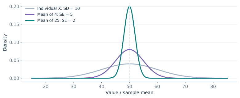
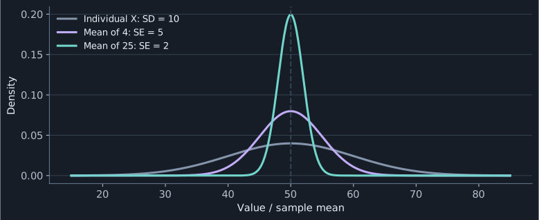
The expectation follows by adding $n$ means and dividing by $n$. For variance, independence allows us to add the $n$ variances, while dividing the sum by $n$ divides its variance by $n^2$. Thus $n\sigma^2/n^2=\sigma^2/n$. Sample means have the same centre as individual observations but less variation.
Key formula
Standard error of a mean
Standard error means the standard deviation of a statistic. It measures the spread of sample means, rather than the spread of individual observations.
4. Exact normal sampling distributions
When the population is normal, any independent sample mean is exactly normal. There is no requirement that the sample size exceed a particular threshold. In the notation $N(\mu,\sigma^2)$, the second parameter is the variance, not the standard deviation.
Key formula
Normal population
The observations must be independent and have this same normal distribution.
Worked example
A sample mean above a threshold
Individual measurements follow $N(50,100)$. For a random independent sample of $25$, find the distribution of $\bar{X}$ and $\operatorname{P}(\bar{X}>54)$.
Divide the population variance by the sample size.
\[\bar{X}\sim N(50,100/25)=N(50,4),\qquad \operatorname{SE}=2\]Standardise using the standard error.
\[\operatorname{P}(\bar{X}>54)=\operatorname{P}\!\left(Z>\frac{54-50}{2}\right)=\operatorname{P}(Z>2)\approx0.0228\]
5. A normal approximation for other populations
The central limit theorem explains why a sample mean can be approximately normal even when individual observations are not. For independent observations from the same population with finite variance, the approximation improves as the sample size increases. Strong skewness or heavy tails may require much larger samples than a nearly symmetric population.
Key formula
Suitable large-sample approximation
Use this only when a normal approximation is suitable. There is no universal rule that $n=30$ guarantees accuracy for every population.
Worked example
A skewed waiting-time population
Waiting times have mean $24$ minutes and standard deviation $10$ minutes. A normal approximation is suitable for the mean of $100$ independent random observations. Estimate $\operatorname{P}(\bar{X}<22)$.
The variance formula still applies although the population is skewed.
\[\operatorname{Var}(\bar{X})=\frac{100}{100}=1,\qquad \operatorname{SE}=1\]Use the stated normal approximation.
\[\operatorname{P}(\bar{X}<22)\approx\operatorname{P}\!\left(Z<\frac{22-24}{1}\right)=\operatorname{P}(Z<-2)\approx0.0228\]
6. Estimating unknown population values
An estimator is unbiased when its expected value equals the parameter it estimates. Since $\operatorname{E}(\bar{X})=\mu$, the sample mean is an unbiased estimator of the population mean. This is a statement about repeated sampling; an individual estimate may still be too high or too low.
Key formula
Unbiased estimate of population variance
Use $n>1$ and an independent sample from a population with finite variance. The variance describing the listed data themselves instead uses denominator $n$.
The deviations from the sample mean sum to zero. Once $n-1$ deviations are known, the last is determined. The denominator $n-1$ also corrects the downward bias caused by measuring deviations from the estimated mean. The square root $s$ estimates the population standard deviation; unbiasedness of $s^2$ does not mean $s$ is itself unbiased.
Worked example
Estimating from raw data
An independent random sample gives $4,6,8,10$. Estimate the population mean and variance, then calculate the estimated standard error of the mean.
Find the observed mean and squared deviations.
\[\bar{x}=7,\qquad\sum(x_i-\bar{x})^2=9+1+1+9=20\]Use the sample-variance denominator.
\[s^2=\frac{20}{3},\qquad s=\sqrt{\frac{20}{3}}\]Divide the estimated standard deviation by the square root of n.
\[\widehat{\operatorname{SE}}=\frac{s}{\sqrt4}=\sqrt{\frac53}\approx1.291\]
7. Choose the appropriate standard error
If the population standard deviation is known, use $\sigma/\sqrt n$. If it is unknown, calculate $s$ from the sample and use the estimated standard error $s/\sqrt n$. Estimating the standard error does not, by itself, justify an exact normal confidence interval or test.
Practice
Try each question before opening its worked solution.
Question 1
A normal population has mean $30$ and variance $16$. For $16$ independent random observations, find the distribution of $\bar{X}$ and $\operatorname{P}(29.5<\bar{X}<31)$.
Show worked solution
Divide the variance by n and take its square root.
\[\bar{X}\sim N(30,16/16)=N(30,1),\qquad \operatorname{SE}=1\]Standardise both endpoints.
\[\operatorname{P}(-0.5<Z<1)=\Phi(1)-\Phi(-0.5)\approx0.8413-0.3085\]
Question 2
For the independent random sample $3,5,5,7$, estimate the population mean, variance and standard error of the sample mean.
Show worked solution
Calculate the mean and sum of squared deviations.
\[\bar{x}=5,\qquad \sum(x_i-\bar{x})^2=4+0+0+4=8\]Use n minus one for variance and the square root of n for standard error.
\[s^2=\frac83,\qquad \widehat{\operatorname{SE}}=\frac{\sqrt{8/3}}{2}=\sqrt{\frac23}\]
Question 3
An independent random sample has $n=10$, $\sum x_i=52$ and $\sum x_i^2=300$. Find $\bar{x}$, $s^2$ and the estimated standard error.
Show worked solution
Use the summarised-data formula.
\[\bar{x}=\frac{52}{10}=5.2,\qquad s^2=\frac{300-52^2/10}{9}=\frac{148}{45}\]Take the square root after dividing the estimated variance by n.
\[\widehat{\operatorname{SE}}=\sqrt{\frac{148/45}{10}}\approx0.5735\]
Question 4
(a) How must sample size change to halve the standard error when $\sigma$ stays fixed? (b) Does this change guarantee that a sample mean from every population is normally distributed?
Show worked solution
Set the new standard error equal to half the old one.
\[\frac{\sigma}{\sqrt{n_{\text{new}}}}=\frac12\frac{\sigma}{\sqrt{n_{\text{old}}}}\quad\Rightarrow\quad n_{\text{new}}=4n_{\text{old}}\]Normality is exact for independent samples from a normal population. For another population, a suitable CLT approximation needs justification.
Use a sampling distribution to assess evidence about a population mean.