Build a numerical probability model and calculate its expectation, variance and probabilities of events.
By the end of this lesson
- Identify the support of a discrete random variable and check a probability distribution.
- Calculate event probabilities, expectations and variances.
- Find expectations of functions and work with a discrete uniform model.
Before you begin: Complements, addition and simple conditional probabilities; Weighted means, squares and square roots.
1. A random variable assigns numbers to outcomes
A random variable is a numerical rule applied to the outcome of a random experiment. We use a capital letter, such as $X$, for the variable and a lower-case letter, such as $x$, for a particular possible value. Before the experiment, $X$ is uncertain; afterwards, an observed value is a number.
For two independent fair coin tosses, define $X$ as the number of heads. The outcomes TT, HT, TH and HH give values $0,1,1,2$. Different outcomes can produce the same value of a random variable.
A discrete random variable has a finite or countably infinite set of possible values. The support consists of the values assigned positive probability. Counts are common examples, but a discrete variable can also take negative values or non-integer values, such as a net profit measured in pounds.
2. A valid probability distribution
A probability distribution lists the possible values together with their probabilities. The probability mass function is $p(x)=P(X=x)$. Probabilities are weights attached to values, so every weight must be nonnegative and the total weight must be exactly one.
Key formula
Validity conditions
The sum covers all possible values. Values outside the support have probability zero.
| $x$ | 0 | 1 | 2 |
|---|---|---|---|
| $P(X=x)$ | $1/4$ | $1/2$ | $1/4$ |
This is the distribution for the number of heads in two fair independent tosses. The probability of one head is $1/2$ because two of the four equally likely coin outcomes produce that value. The three numerical values of $X$ are therefore not equally likely.
3. Event probabilities and unknown constants
To find the probability of an event, add the probabilities of all values that satisfy it. Pay attention to endpoints. For integer-valued $X$, the events $X>1$ and $X\ge2$ are the same, but $X\ge1$ also includes the value $1$.
Key formula
Adding the relevant masses
A is any specified set of values. Include only values allowed by the distribution.
The identity $P(X\ge1)=1-P(X=0)$ applies when $X$ is a non-negative integer-valued variable. If negative values are possible, the complementary event is $X<1$, which may contain more than just zero.
Worked example
Finding a normalising constant
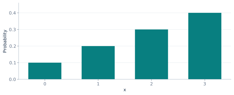
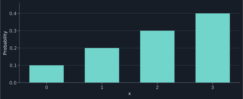
A variable has values $0,1,2,3$ with probabilities $k,2k,3k,4k$, respectively. Find $k$ and $P(X\ge2)$.
The four probabilities must sum to one.
\[k+2k+3k+4k=10k=1\]Solve for the constant and check that every resulting probability is nonnegative.
\[k=0.1\]The event includes the values 2 and 3.
\[P(X\ge2)=3k+4k=0.7\]
4. Expectation is a probability-weighted mean
The expectation $\operatorname{E}(X)$ describes the theoretical mean of the model. Multiply each possible value by its probability, then add. This has the same structure as a frequency-weighted mean, but the probability weights already sum to one.
Key formula
Expected value
For a finite distribution, sum all its values. For an infinite distribution, the required expectation must exist.
In repeated independent trials of the same model, the average observed value tends towards the expectation under the usual finite-mean conditions. The expectation need not occur in any single trial. A fair die has expectation $3.5$, although a die never displays $3.5$.
The most likely value is the mode, not necessarily the expectation. In the distribution $0,1,2,3$ with probabilities $0.1,0.2,0.3,0.4$, the mode is $3$, while the expectation is $2$.
5. The second moment and variance
The second moment, $\operatorname{E}(X^2)$, is the weighted mean of the squared values. Square each value before multiplying by its probability. It is generally different from the square of the expectation.
Key formula
Variance and standard deviation
Assume the second moment is finite. Variance is nonnegative and has squared units; standard deviation has the same unit as X.
Worked example
Calculating two moments
For $x=0,1,2,3$ with probabilities $0.1,0.2,0.3,0.4$, find the expectation, variance and standard deviation.
Weight each value by its probability.
\[\operatorname{E}(X)=0(0.1)+1(0.2)+2(0.3)+3(0.4)=2\]Weight each squared value by the same probability.
\[\operatorname{E}(X^2)=0^2(0.1)+1^2(0.2)+2^2(0.3)+3^2(0.4)=5\]Subtract the square of the first moment, then take a square root.
\[\operatorname{Var}(X)=5-2^2=1,\qquad\operatorname{SD}(X)=1\]
Variance measures spread around the expected value. It can also be written as $\operatorname{E}[(X-\mu)^2]$. If your calculation gives a negative variance, check the probabilities, the squared values and the order of subtraction.
6. Uniform models and functions of a variable
A discrete uniform variable gives equal probability to each value in a finite support. If there are $m$ values, each has probability $1/m$. “Uniform” refers to the equal probabilities; the possible numerical values still need to be stated.
Worked example
A fair four-score spinner
A fair spinner has scores $1,2,3,4$. Find the mean and variance of its score $S$.
Each score has probability one quarter.
\[\operatorname{E}(S)=\frac{1+2+3+4}{4}=2.5\]Calculate the second moment.
\[\operatorname{E}(S^2)=\frac{1+4+9+16}{4}=7.5\]Subtract the square of the expectation.
\[\operatorname{Var}(S)=7.5-2.5^2=1.25\]
Sometimes the quantity of interest is a function $g(X)$, such as a payoff or a squared distance. Apply the function to each possible value first, then average using the original probabilities.
Key formula
Expectation of a function
The expectation must exist. In general, this is different from $g[\operatorname{E}(X)]$.
For the two-coin variable, let $g(X)=(X-1)^2$. Its transformed values are $1,0,1$, so $\operatorname{E}[g(X)]=1(1/4)+0(1/2)+1(1/4)=1/2$. But $\operatorname{E}(X)=1$ gives $g[\operatorname{E}(X)]=0$. Nonlinear transformations usually prevent interchanging the function and the expectation.
Practice
Try each question before opening its worked solution.
Question 1
$X$ takes values $-1,0,2$ with probabilities $0.2,0.5,0.3$. Find its expectation, variance and standard deviation.
Show worked solution
Calculate the two moments.
\[\operatorname{E}(X)=-1(0.2)+0(0.5)+2(0.3)=0.4\]The negative value becomes positive when squared.
\[\operatorname{E}(X^2)=1(0.2)+0(0.5)+4(0.3)=1.4\]Find variance and its square root.
\[\operatorname{Var}(X)=1.4-0.4^2=1.24,\qquad\operatorname{SD}(X)\approx1.11\]
Question 2
$Y$ takes values $0,1,2$ with probabilities $0.2,0.3,k$. Find $k$, $\operatorname{E}(Y)$ and $\operatorname{Var}(Y)$.
Show worked solution
Use the total-probability condition.
\[k=1-0.2-0.3=0.5\]Calculate the first and second moments.
\[\operatorname{E}(Y)=0.3+2(0.5)=1.3,\qquad\operatorname{E}(Y^2)=0.3+4(0.5)=2.3\]Calculate variance.
\[\operatorname{Var}(Y)=2.3-1.3^2=0.61\]
Question 3
$Z$ is uniform on $\{1,2,3,4,5,6\}$. Find $P(Z\ge5)$, its expectation and its variance.
Show worked solution
Two of the six equally likely values satisfy the event.
\[P(Z\ge5)=\frac26=\frac13\]Average the values and their squares.
\[\operatorname{E}(Z)=\frac{21}{6}=3.5,\qquad\operatorname{E}(Z^2)=\frac{91}{6}\]Keep the fraction exact until the final subtraction.
\[\operatorname{Var}(Z)=\frac{91}{6}-\left(\frac72\right)^2=\frac{35}{12}\]
Question 4
A game has score $X=0,1,2$ with probabilities $0.5,0.3,0.2$. Its net payoff in pounds is $Y=3X-2$. Find the expected net payoff and the probability of making a profit.
Show worked solution
Transform each score to obtain net payoffs of −2, 1 and 4 pounds.
\[\operatorname{E}(Y)=(-2)(0.5)+1(0.3)+4(0.2)=0.1\]A profit occurs when the net payoff is positive, which corresponds to scores 1 and 2.
\[P(Y>0)=0.3+0.2=0.5\]
The binomial model gives a formula for the distribution of a count of successes in independent repeated trials.