Continuous random variables — chapter review — 9231 FPS
Integrate on the correct branch and keep a cumulative distribution continuous. Find a transformed distribution through its CDF and support. Normalise a density and compute probabilities and moments by integration.
Notes and key methods
Normalise a piecewise density by adding its separate integrals. The cumulative distribution \(F(x)=P(X\le x)\) must include all area to the left, including completed earlier pieces.
For an absolutely continuous variable, F is continuous, nondecreasing, zero below the support and one above it. At a point where f changes formula, match the two CDF expressions rather than resetting the accumulated probability.
To find the distribution of \(\displaystyle Y=g(X)\), first determine its support and write \(F_Y(y)=P(g(X)\le y)\). On a monotone increasing branch, invert g to obtain \(F_X(g^{-1}(y))\), then differentiate.
A decreasing transformation reverses the inequality. If g is not one-to-one, collect every inverse branch that contributes. The Jacobian formula uses the absolute derivative of the inverse.
A density f is nonnegative and integrates to one over its support. Probabilities are areas: \(P(a<X<b)=\int_a^b f(x)\,dx\). A density may be larger than 1; a probability cannot.
Use \(E(X)=\int xf(x)\,dx\), \(E(X^2)=\int x^2f(x)\,dx\) and \(\operatorname{Var}(X)=E(X^2)-E(X)^2\). A median m solves \(\displaystyle \int_{- \infty }^{m} f(x)\, dx= \frac{1}{2}\).
Check the conditions
Integrate separately across every density breakpoint.
A continuous density model has no positive point masses at breakpoints.
A single inverse branch is valid only on a monotone support.
The new support must be stated before integrating or differentiating.
State the full support and put \(\displaystyle f(x)=0\) outside it.
The density must be nonnegative throughout its support.
Three worked examples
Example 1 · Piecewise densities and cumulative functions
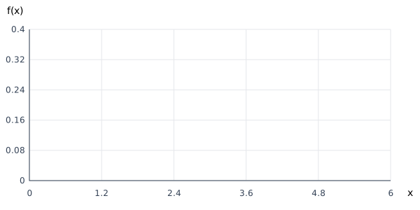
The density is \(f(x)=kx\ (0\le x\le 3),\quad f(x)=k(6-x)\ (3<x\le 6)\), and zero elsewhere.
Use the labelled scales alongside the numerical method.
Example 2 · Transformations of continuous variables
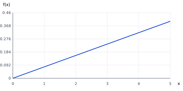
X has density \(\displaystyle \frac{2x}{16}\) on \(0\le x\le 4\). Define \(\displaystyle Y=X^{2}\). For \(0\le y\le 16\), \(\displaystyle F_{Y}(y)= P(X\le \sqrt{y})= \frac{y}{16}\).