Maths4U
Menu

Maths4U Original · Learn, check, explain

Stationary points and classification — 0606

Locate stationary points and justify their nature.

Notes and key methods

A differentiable curve has a stationary point where \(\displaystyle f'(x)=0\). Solve for the abscissae, then find the ordinates using f, not f′. If f″(a)>0 there is a local minimum; if f″(a)<0 there is a local maximum.

If f″\(\displaystyle (a)=0\), this test is inconclusive: inspect the sign of f′ on both sides or use further reasoning. A stationary inflection is neither a maximum nor a minimum.

Check the conditions

Three worked examples

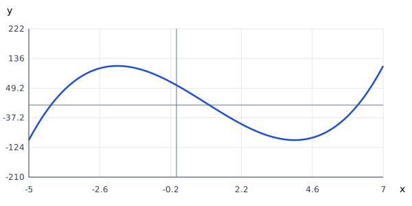
Example 1 · Stationary points and second derivatives

Consider \(y=- 12 x + \left(x - 5\right)^{3} + 65\).

Diagram for this worked example
Use the labelled scales alongside the numerical method.
  1. Find both stationary points.
  2. Classify both stationary points with justification.
  3. Find the height of the local maximum.
  4. Find the height of the local minimum.
Show the reasoning

(a)

\(3 \left(x - 5\right)^{2} - 12\) vanishes at \(3\) and \(7\). Substitute each into f.

Answer: \(\left( 3, \ 21\right)\) and \(\left( 7, \ -11\right)\)

(b)

The second derivative is \(6 \left(x - 5\right)\). Its values are \(-12\) and \(12\), respectively.

Answer: The first is a local maximum; the second is a local minimum.

(c)

Evaluate f at h−d; the second derivative is negative.

\(21\)

Answer: \(21\).

(d)

Evaluate f at h+d; the second derivative is positive.

\(-11\)

Answer: \(-11\).

Example 2 · Stationary points and second derivatives
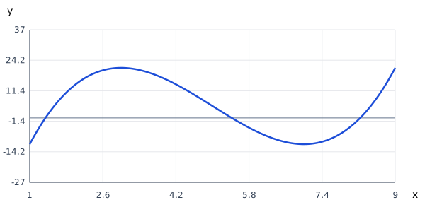
Consider \(y=- 54 x + 2 \left(x - 1\right)^{3} + 60\).

Diagram for this worked example
Use the labelled scales alongside the numerical method.
  1. Find both stationary points.
  2. Classify both stationary points with justification.
  3. Find the height of the local maximum.
  4. Find the height of the local minimum.
Show the reasoning

(a)

\(6 \left(x - 1\right)^{2} - 54\) vanishes at \(-2\) and \(4\). Substitute each into f.

Answer: \(\left( -2, \ 114\right)\) and \(\left( 4, \ -102\right)\)

(b)

The second derivative is \(12 \left(x - 1\right)\). Its values are \(-36\) and \(36\), respectively.

Answer: The first is a local maximum; the second is a local minimum.

(c)

Evaluate f at h−d; the second derivative is negative.

\(114\)

Answer: \(114\).

(d)

Evaluate f at h+d; the second derivative is positive.

\(-102\)

Answer: \(-102\).

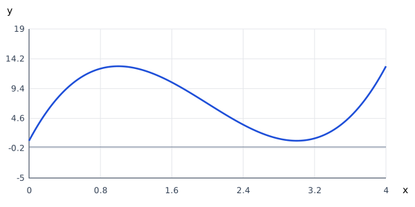
Example 3 · Stationary points and second derivatives
Consider \(y=- 9 x + 3 \left(x - 2\right)^{3} + 25\).

Diagram for this worked example
Use the labelled scales alongside the numerical method.
  1. Find both stationary points.
  2. Classify both stationary points with justification.
  3. Find the height of the local maximum.
  4. Find the height of the local minimum.
Show the reasoning

(a)

\(9 \left(x - 2\right)^{2} - 9\) vanishes at \(1\) and \(3\). Substitute each into f.

Answer: \(\left( 1, \ 13\right)\) and \(\left( 3, \ 1\right)\)

(b)

The second derivative is \(18 \left(x - 2\right)\). Its values are \(-18\) and \(18\), respectively.

Answer: The first is a local maximum; the second is a local minimum.

(c)

Evaluate f at h−d; the second derivative is negative.

\(13\)

Answer: \(13\).

(d)

Evaluate f at h+d; the second derivative is positive.

\(1\)

Answer: \(1\).

Common mistakes

Practise with answer checking

Original exam-style problems

Write complete solutions before opening the worked solution. The marking guidance rewards reasoning as well as answers.

Examination practice · 2020–2026

Apply the method to recent source-labelled questions from this chapter.

Browse recent examination questions · All topic resources and the full bank

Next skill: Practical maximum and minimum problems →