0580 P21 - Jun 2026 - Q14 - 5 marks
The cumulative frequency graph represents the television watching times of 60 students on one day.
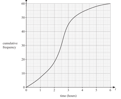
(a(i)) Estimate the median watching time. [1]
(a(ii)) Estimate the interquartile range. [2]
(b) Complete the two missing frequencies in the table. [2]
| Time \(t\) (hours) | \(0<t\le1\) | \(1<t\le2\) | \(2<t\le3\) | \(3<t\le4\) | \(4<t\le5\) | \(5<t\le6\) |
|---|---|---|---|---|---|---|
| Frequency | 7 | 9 | 4 | 2 |

0580 P21 - Jun 2025 - Q12 - 4 marks
The time spent on the internet by each of 120 adults is recorded for one day. The cumulative frequency diagram gives the results.
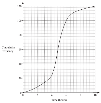
(a) Estimate the interquartile range. [2]
(b) \(70\%\) of the adults spent less than k hours on the internet. Estimate k. [2]

0580 P43 - Jun 2025 - Q19 - 4 marks
The cumulative frequency table shows the heights of 200 plants.
| Height (cm) | Cumulative frequency |
|---|---|
| \(h\le30\) | 6 |
| \(h\le40\) | 42 |
| \(h\le50\) | 76 |
| \(h\le60\) | 170 |
| \(h\le70\) | 190 |
| \(h\le80\) | 200 |
(a) Draw a cumulative frequency diagram. [3]
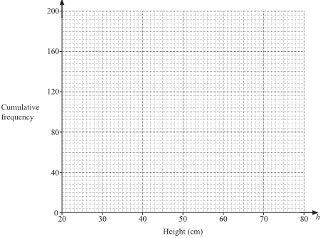
(b) Estimate the 75th percentile. [1]


0580 P23 - Jun 2024 - Q15 - 4 marks
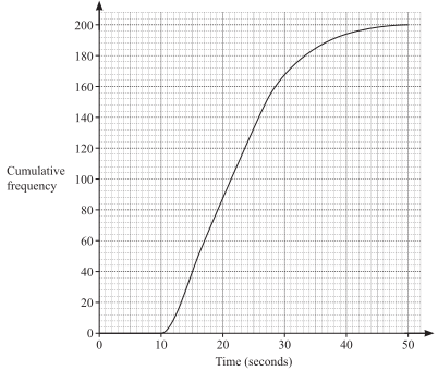
The graph shows the times taken by 200 students to complete a calculation. Use it to estimate:
(a) the interquartile range; [2]
(b) the number taking more than 40 seconds. [2]

0580 P41 - Jun 2023 - Q5 - 13 marks
The cumulative frequency graph shows ages of 160 people in a village.


Ages in another village are grouped as follows.
| Age \(n\) (years) | \(0<n\le20\) | \(20<n\le30\) | \(30<n\le50\) | \(50<n\le80\) |
|---|---|---|---|---|
| Frequency | 52 | 37 | 24 | 60 |

(a(i)(a)) Estimate the median age. [1]
(a(i)(b)) Estimate the lower quartile. [1]
(a(i)(c)) Estimate how many people are 50 years old or older. [2]
(a(i)(d)) Estimate the 65th percentile. [2]
(a(ii)(a)) The youngest is 1 and oldest 70. Draw a box-and-whisker plot for the ages. [3]
(a(ii)(b)) Estimate the percentage younger than the median. [1]
(b) Complete the histogram for the other village. [3]


0580 P42 - Jun 2023 - Q4 - 18 marks
The table gives heights of 80 children.
| Height \(h\) (m) | \(1.2<h\le1.4\) | \(1.4<h\le1.5\) | \(1.5<h\le1.65\) | \(1.65<h\le1.8\) | \(1.8<h\le1.9\) |
|---|---|---|---|---|---|
| Frequency | 2 | 13 | 24 | 32 | 9 |

(a(i)) Write the interval containing the median. [1]
(a(ii)) Estimate the mean height. [4]
(b(i)) One child is chosen at random. Find the probability their height is 1.4 m or less. [1]
(b(ii)) Two children are chosen at random without replacement. Find the probability both are taller than 1.5 m but only one is taller than 1.8 m. [3]
(c(i)) Complete the cumulative frequency table at heights 1.4, 1.5, 1.65, 1.8 and 1.9 m; the first cumulative frequency is 2. [2]
(c(ii)) Draw the cumulative frequency diagram. [3]
(d(i)) Use your diagram to estimate the interquartile range. [2]
(d(ii)) Use your diagram to estimate the 60th percentile. [2]


0580 P43 - Jun 2023 - Q6 - 15 marks
A speed camera records 200 cars.
| Speed \(v\) (km/h) | \(v\le70\) | \(v\le80\) | \(v\le90\) | \(v\le95\) | \(v\le100\) | \(v\le120\) |
|---|---|---|---|---|---|---|
| Cumulative frequency | 12 | 46 | 115 | 155 | 177 | 200 |

Masses of 50 trucks are grouped below.
| Mass \(m\) (kg) | \(2000<m\le2600\) | \(2600<m\le3500\) | \(3500<m\le5000\) | \(5000<m\le5700\) |
|---|---|---|---|---|
| Frequency | 12 | 15 | 16 | 7 |
(a(i)) Draw the cumulative frequency diagram for speeds. [3]
(a(ii)(a)) Estimate the median speed from your graph. [1]
(a(ii)(b)) Estimate the interquartile range. [2]
(a(ii)(c)) Estimate the number of cars with speed greater than 110 km/h. [2]
(b(i)) Estimate the mean truck mass. [4]
(b(ii)) The first block of a truck-mass histogram is 6 cm high. Find the heights of the next three blocks, in order. [3]


0580 P42 - Mar 2022 - Q5 - 18 marks
Masses of 120 letters:
| Mass (g) | \(0<m\le50\) | \(50<m\le100\) | \(100<m\le200\) | \(200<m\le500\) |
|---|---|---|---|---|
| Frequency | 43 | 31 | 25 | 21 |

(a) Estimate the mean mass. [4]
(b) A histogram’s first bar is 17.2 cm high. Find the remaining three bar heights. [3]
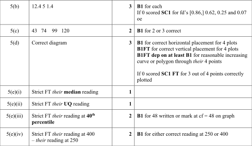
(c) Complete cumulative frequencies at 50, 100, 200 and 500 g. [2]
(d) Draw a cumulative frequency diagram. [3]
(e(i)) Use your diagram to estimate the median. [1]
(e(ii)) Estimate the upper quartile. [1]
(e(iii)) Estimate the 40th percentile. [2]
(e(iv)) Estimate how many letters have \(250<m\le400\). [2]


0580 P43 - Jun 2022 - Q5 - 19 marks
Times to work for 80 people:
| Time \(t\) (min) | \(0<t\le5\) | \(5<t\le10\) | \(10<t\le20\) | \(20<t\le35\) | \(35<t\le60\) |
|---|---|---|---|---|---|
| Frequency | 3 | 7 | 18 | 28 | 24 |
(a(i)) State the class interval containing the median. [1]
(a(ii)) Estimate the mean time. [4]
(b(i)) Choose one person. Find the probability their time exceeded 10 minutes as a fraction in simplest form. [2]
(b(ii)) Choose two from those taking at most 20 minutes. Find the probability one took at most 5 minutes and the other more than 5. [3]
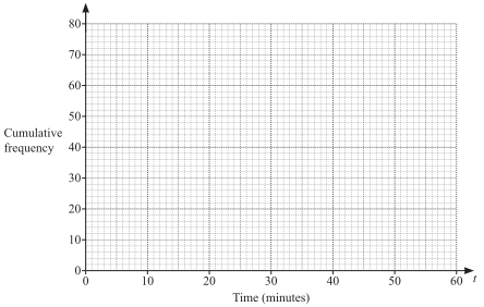
(c(i)) Complete cumulative frequencies at 5, 10, 20, 35 and 60 minutes; 3, 10 and 80 are given. [1]
(c(ii)) Draw a cumulative frequency diagram. [3]
(c(iii)) Estimate the 80th percentile. [2]
(c(iv)) Estimate the percentage taking more than 45 minutes, showing working. [3]


0580 P22 - Nov 2022 - Q13 - 4 marks
| Mass k (kg) | 20 | 22 | 24 | 28 | 32 | 36 | 42 |
|---|---|---|---|---|---|---|---|
| Cumulative frequency | 0 | 7 | 23 | 35 | 43 | 47 | 50 |
(a) Draw a cumulative frequency diagram. [3]
(b) Use it to estimate the 90th percentile. [1]


0580 P41 - Nov 2022 - Q5 - 14 marks

100 students record their time t to eat a pizza. Separately, 150 students record tennis-ball throwing distances:
| Distance d (m) | \(0<d\le20\) | \(20<d\le30\) | \(30<d\le35\) | \(35<d\le45\) | \(45<d\le60\) |
|---|---|---|---|---|---|
| Frequency | 4 | 38 | 40 | 53 | 15 |
(a(i)) Estimate the median pizza-eating time. [1]
(a(ii)) Estimate its interquartile range. [2]
(a(iii)) Estimate the number taking more than 11 minutes. [2]
(b(i)) Estimate the mean throwing distance. [4]
(b(ii)) In a histogram the bar for \(30<d\le35\) is 12 cm high. Find each other bar height. [3]
(b(iii)) Choose two students at random. Find the probability both threw more than 45 m. [2]

0580 P41 - Jun 2021 - Q8 - 10 marks
Masses of 50 children:
| Mass k (kg) | 0 < k ≤ 10 | 10 < k ≤ 25 | 25 < k ≤ 35 | 35 < k ≤ 40 | 40 < k ≤ 50 |
|---|---|---|---|---|---|
| Frequency | 3 | 19 | 21 | 5 | 2 |


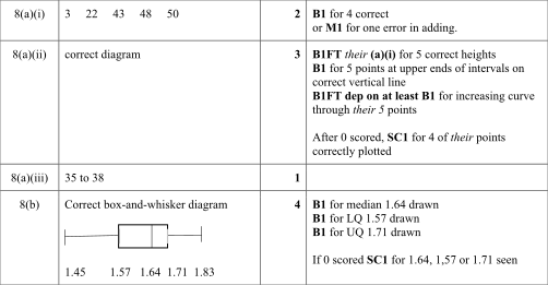
(a(i)) Complete the cumulative frequencies at 10, 25, 35, 40, 50 kg. [2]
(a(ii)) Draw the cumulative frequency diagram for the masses. [3]
(a(iii)) Use the diagram to estimate the number weighing 32 kg or less. [1]
(b) For the height diagram, shortest height is 1.45 m and tallest is 1.83 m. Draw a box-and-whisker plot. [4]

0580 P41 - Nov 2021 - Q3 - 16 marks
The cumulative frequency diagram shows masses m kg of 80 boys.

(a) Draw a box-and-whisker plot of these data. [4]
(b(i)) Estimate the 30th percentile. [2]
(b(ii)) Estimate the number with mass greater than 75 kg. [2]
(c(i)) Complete the missing frequencies below. [1]
(c(ii)) Estimate the mean mass. [4]
(c(iii)) Two boys are randomly selected without replacement from those heavier than 70 kg. Find the probability that one is heavier than 80 kg and the other is at most 80 kg. [3]
| Mass (kg) | \(30<m\le40\) | \(40<m\le50\) | \(50<m\le60\) | \(60<m\le70\) | \(70<m\le80\) | \(80<m\le90\) |
|---|---|---|---|---|---|---|
| Frequency | 8 | 12 | … | … | 14 | 10 |


0580 P42 - Nov 2021 - Q2 - 16 marks
The cumulative frequency diagram shows the floor areas of 80 houses.

| Floor area (m²) | \(40<a\le60\) | \(60<a\le80\) | \(80<a\le100\) | \(100<a\le130\) | \(130<a\le160\) | \(160<a\le200\) |
|---|---|---|---|---|---|---|
| Frequency | 14 | 17 | 18 | 15 | 9 | 7 |
(a(i)) Estimate the median. [1]
(a(ii)) Estimate the lower quartile. [1]
(a(iii)) Estimate the interquartile range. [1]
(a(iv)) Estimate the number of houses with area greater than 120 m². [2]
(b(i)) Estimate the mean floor area using the table. [4]
(b(ii)) Draw the histogram for these data. [4]
(b(iii)) Two houses are chosen at random without replacement. Find the probability that one has area greater than 130 m² and the other at most 60 m². [3]


0580 P41 - Jun 2020 - Q2 - 18 marks
The heights h metres of 120 boys in an athletics club are recorded.
| Height | \(1.3<h\le1.4\) | \(1.4<h\le1.5\) | \(1.5<h\le1.6\) | \(1.6<h\le1.7\) | \(1.7<h\le1.8\) | \(1.8<h\le1.9\) |
|---|---|---|---|---|---|---|
| Frequency | 7 | 18 | 30 | 24 | 27 | 14 |
(a(i)) State the modal class. [1]
(a(ii)) Estimate the mean height. [4]
(b(i)) One boy is selected randomly. Find the probability his height exceeds 1.8 m. [1]
(b(ii)) Three boys are selected randomly without replacement. Find the probability that exactly one has height greater than 1.8 m and the other two each have height 1.4 m or less. [4]
(c(i)) Complete the cumulative frequency table.
| Height | \(h\le1.4\) | \(h\le1.5\) | \(h\le1.6\) | \(h\le1.7\) | \(h\le1.8\) | \(h\le1.9\) |
|---|---|---|---|---|---|---|
| Cumulative frequency | 7 | 25 | … | … | … | … |
(c(ii)) Draw a cumulative frequency diagram. [3]
(d(i)) Use the diagram to estimate the median height. [1]
(d(ii)) Use the diagram to estimate the 40th percentile. [2]


0580 P42 - Jun 2020 - Q3 - 16 marks
The speed v km/h of 200 cars is measured.
| Speed | \(0<v\le20\) | \(20<v\le40\) | \(40<v\le45\) | \(45<v\le50\) | \(50<v\le60\) | \(60<v\le80\) |
|---|---|---|---|---|---|---|
| Frequency | 16 | 34 | 62 | 58 | 26 | 4 |
(a) Estimate the mean speed. [4]
(b(i)) Complete the cumulative frequency table.
| Speed | \(v\le20\) | \(v\le40\) | \(v\le45\) | \(v\le50\) | \(v\le60\) | \(v\le80\) |
|---|---|---|---|---|---|---|
| Cumulative frequency | 16 | 50 | … | … | 196 | 200 |
(b(ii)) Draw a cumulative frequency diagram. [3]
(b(iii)(a)) Use the diagram to estimate the upper quartile. [1]
(b(iii)(b)) Use the diagram to estimate how many cars have speed greater than 35 km/h. [2]
(c) Choose two of the 200 cars randomly without replacement. Find the probability both have speed greater than 50 km/h. [2]
(d) Draw a histogram for the combined intervals.
| Speed | \(0<v\le40\) | \(40<v\le50\) | \(50<v\le80\) |
|---|---|---|---|
| Frequency | 50 | 120 | 30 |


0580 P42 - Nov 2020 - Q4 - 12 marks
The heights h cm of 120 plants are shown by the cumulative frequency graph.

(a(i)) Estimate the median. [1]
(a(ii)) Estimate the interquartile range. [2]
(a(iii)) Estimate the 60th percentile. [1]
(a(iv)) Estimate the number taller than 40 cm. [2]
| Height (cm) | \(0<h\le10\) | \(10<h\le20\) | \(20<h\le30\) | \(30<h\le50\) |
|---|---|---|---|---|
| Frequency | 2 | 18 | 62 | 38 |
(b(i)) Estimate the mean height. [4]
(b(ii)) In a histogram, the bar for \(10<h\le20\) is 7.2 cm high. Find the height for \(30<h\le50\). [2]

0580 P23 - Jun 2019 - Q23 - 5 marks
160 students record their weekly computer gaming time t hours.

(a(i)) Estimate the median. [1]
(a(ii)) Estimate the interquartile range. [2]
(b) Complete the frequency table. [2]
| Time t (hours) | Frequency |
|---|---|
| 0<t≤2 | 20 |
| 2<t≤4 | … |
| 4<t≤6 | … |
| 6<t≤8 | 24 |
| 8<t≤10 | 12 |
| 10<t≤12 | 4 |

0580 P42 - Jun 2019 - Q9 - 14 marks
100 students record weekly spending \$m:
| Amount m (\$) | Frequency |
|---|---|
| 0<m≤5 | 16 |
| 5<m≤10 | 38 |
| 10<m≤20 | 30 |
| 20<m≤30 | 9 |
| 30<m≤50 | 7 |
(a) Estimate the mean. [4]
(b) Complete the cumulative frequencies for m≤5,10,20,30,50, with first16 and last100. [2]
(c) Draw the cumulative frequency diagram. [3]

(d(i)) Estimate the median. [1]
(d(ii)) Estimate the interquartile range. [2]
(d(iii)) Estimate the number spending more than \$25. [2]


0580 P41 - Nov 2019 - Q6 - 17 marks
The cumulative frequency diagram shows times taken by 200 students to solve a problem.

(a(i)) Estimate the median. [1]
(a(ii)) Estimate the interquartile range. [2]
(a(iii)) Estimate how many took more than 40 minutes. [2]
Roberto records the values of his coins.
| Value (cents) | 1 | 2 | 5 | 10 | 20 | 50 |
|---|---|---|---|---|---|---|
| Frequency | 3 | 1 | 3 | 2 | 4 | 2 |
(b(i)) Find the range. [1]
(b(ii)) Find the mode. [1]
(b(iii)) Find the median. [1]
(b(iv)) Find the total value. [2]
(b(v)) Find the mean. [1]
The histogram shows the masses of 100 boxes.

(c) Estimate the mean mass. [6]


0580 P42 - Nov 2019 - Q2 - 15 marks
The cumulative frequency diagram shows times for a group of girls to solve a maths problem.

(a(i)) Estimate the median. [1]
(a(ii)) Estimate the interquartile range. [2]
(a(iii)) Estimate the 20th percentile. [1]
(a(iv)) Estimate the number taking more than 66 seconds. [2]
| Time t (seconds) | \(0<t\le20\) | \(20<t\le40\) | \(40<t\le60\) | \(60<t\le80\) | \(80<t\le100\) |
|---|---|---|---|---|---|
| Frequency | 6 | … | … | … | 4 |
(b(i)) Complete the frequency table using the diagram. [2]
(b(ii)) Estimate the mean time. [4]
Boys solving the same problem have median 60 s, lower quartile 46 s and upper quartile 66 s.
(c(i)) What percentage of boys took 66 s or less? [1]
(c(ii)) Howard says the boys’ times vary more. Explain why he is incorrect. [2]

0580 P43 - Nov 2019 - Q5 - 12 marks
The cumulative frequency diagram shows weekend distances of 60 male cyclists.

(a(i)) Estimate the median. [1]
(a(ii)) Estimate the lower quartile. [1]
(a(iii)) Estimate the interquartile range. [1]
(b) The female cyclists’ IQR is 40 km. Compare the distributions. [1]
(c) Find the probability that a randomly chosen male cyclist travelled more than 50 km. [2]
| Distance d (km) | Number |
|---|---|
| \(0<d\le40\) | 18 |
| \(40<d\le50\) | 9 |
| \(50<d\le60\) | … |
| \(60<d\le70\) | … |
| \(70<d\le90\) | … |
| \(90<d\le120\) | 2 |
(d(i)) Complete the frequency table using the graph. [2]
(d(ii)) Estimate the mean distance. [4]


0580 P42 - Mar 2018 - Q7 - 17 marks
Times of 160 library visitors are recorded.
| Time m (minutes) | \(0<m\le10\) | \(10<m\le40\) | \(40<m\le60\) | \(60<m\le90\) | \(90<m\le100\) | \(100<m\le120\) |
|---|---|---|---|---|---|---|
| Frequency | 3 | 39 | 43 | 55 | 11 | 9 |
(a(i)) Find the probability of spending more than 100 minutes. [1]
(a(ii)) Estimate the mean time. [4]
| m≤ | 10 | 40 | 60 | 90 | 100 | 120 |
|---|---|---|---|---|---|---|
| Cumulative frequency | 3 | 42 | … | … | … | … |
(b) Complete the cumulative table. [2]

(c) Draw the cumulative frequency diagram. [3]
(d(i)) Use it to estimate the median. [1]
(d(ii)) Estimate the interquartile range. [2]
(d(iii)) Estimate the 90th percentile. [2]
(d(iv)) Estimate how many spent more than 30 minutes. [2]


0580 P21 - Jun 2018 - Q18 - 4 marks
The cumulative frequency graph shows the time m minutes taken by 120 students to complete homework.

(a) Estimate the interquartile range. [2]
(b) Estimate how many students took more than 50 minutes. [2]

0580 P42 - Jun 2018 - Q2 - 17 marks
Cooking challenge times for 120 students:
| t (minutes) | \(20<t\le25\) | \(25<t\le30\) | \(30<t\le35\) | \(35<t\le40\) | \(40<t\le45\) |
|---|---|---|---|---|---|
| Frequency | 44 | 32 | 28 | 12 | 4 |
(a(i)) State the modal interval. [1]
(a(ii)) State the interval containing the median. [1]
(a(iii)) Estimate the mean time. [4]
(a(iv)) Find the probability a randomly chosen student takes more than 40 minutes. [1]
| Time | \(t\le20\) | \(t\le25\) | \(t\le30\) | \(t\le35\) | \(t\le40\) | \(t\le45\) |
|---|---|---|---|---|---|---|
| Cumulative frequency | 0 | 44 | ____ | ____ | ____ | ____ |
(b(i)) Complete the cumulative frequency table. [2]
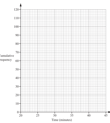
(b(ii)) Draw a cumulative frequency diagram. [3]
(b(iii)) Find the median time. [1]
(b(iv)) Find the interquartile range. [2]
(b(v)) Find how many took more than 37 minutes. [2]


0580 P22 - Nov 2018 - Q24 - 5 marks
The diagram shows homework times t minutes for 80 students.

(a) Estimate the median. [1]
(b) Estimate the interquartile range. [2]
(c) Estimate how many take more than 40 minutes. [2]

0580 P41 - Nov 2018 - Q4 - 18 marks
Heights h cm of 180 children:
| Height | 60| 70 | 90 | 100 | 110 | 115 | |
|---|---|---|---|---|---|---|
| Frequency | 8 | 26 | 35 | 67 | 28 | 16 |
(a) Estimate the mean to 1 decimal place. [4]
(b) In a histogram, the 60<h≤70 bar is 0.4 cm high. Find heights for 115<h≤125,110<h≤115,70<h≤90. [3]
(c) Complete cumulative frequencies at 70,90,100,110,115,125 (last value 180). [2]

(d) Draw a cumulative frequency diagram. [3]
(e(i)) Estimate the interquartile range. [2]
(e(ii)) Estimate the 70 th percentile. [2]
(e(iii)) Estimate the number taller than 106 cm. [2]


0580 P42 - Mar 2017 - Q7 - 14 marks
Times taken by 400 people to complete a race:
| Time m (minutes) | \(45<m\le50\) | \(50<m\le60\) | \(60<m\le70\) | \(70<m\le90\) | \(90<m\le100\) | \(100<m\le120\) |
|---|---|---|---|---|---|---|
| Frequency | 23 | 64 | 122 | 136 | 26 | 29 |
(a) Estimate the mean time. [4]
(b(i)) Complete cumulative frequencies for m≤50,60,70,90,100,120; the first is 23 and last 400. [2]

(b(ii)) Draw the cumulative frequency diagram. [3]
Use the diagram to estimate
(b(iii)(a)) the median; [1]
(b(iii)(b)) the interquartile range; [2]
(b(iii)(c)) the 60 th percentile. [2]


0580 P41 - Jun 2017 - Q2 - 17 marks
Lap times for 90 cars are shown.
| t (seconds) | \(70<t\le71\) | \(71<t\le72\) | \(72<t\le73\) | \(73<t\le74\) | \(74<t\le75\) |
|---|---|---|---|---|---|
| Frequency | 17 | 24 | 21 | 18 | 10 |
(a) Write the modal interval. [1]
(b) Estimate the mean time. [4]
| Time | \(t\le71\) | \(t\le72\) | \(t\le73\) | \(t\le74\) | \(t\le75\) |
|---|---|---|---|---|---|
| Cumulative frequency | 17 |
(c(i)) Complete the cumulative frequency table. [2]

(c(ii)) Draw a cumulative frequency diagram. [3]
(c(iii)) Find the median time. [1]
(c(iv)) Find the interquartile range. [2]
(d) The lap measures 3720 m, correct to the nearest 10 m. A car completed it in 75 s, correct to the nearest second. Find the upper bound for average speed in km/h. [4]


0580 P21 - Nov 2017 - Q22 - 7 marks
Simon records the heights of 200 sunflowers.

(a) Find how many sunflowers are taller than 160 cm. [2]
Sue records 200 sunflowers:
| Height h (cm) | \(h\le100\) | \(h\le110\) | \(h\le120\) | \(h\le130\) | \(h\le140\) | \(h\le150\) | \(h\le160\) | \(h\le170\) |
|---|---|---|---|---|---|---|---|---|
| Cumulative frequency | 0 | 20 | 48 | 100 | 140 | 172 | 188 | 200 |
(b) Draw Sue’s cumulative frequency graph on the same grid. [3]
(c) Find the difference between the median heights. [2]


0580 P42 - Mar 2016 - Q4 - 14 marks
The cumulative frequency curve shows the times \(t\) minutes taken by 60 students to finish a test.

(a(i)) Estimate the median time. [1]
(a(ii)) Estimate the inter-quartile range. [2]
(a(iii)) Estimate the 40th percentile. [2]
(a(iv)) Find how many students took more than 80 minutes. [2]
| Time (min) | \(0<t\le40\) | \(40<t\le60\) | \(60<t\le70\) | \(70<t\le80\) | \(80<t\le90\) | \(90<t\le100\) |
|---|---|---|---|---|---|---|
| Frequency | 8 | 4 |
(b) Complete the frequency table using the curve. [3]

(c) Complete the histogram for your frequency table. [4]


0580 P23 - Jun 2016 - Q22 - 6 marks
The cumulative frequency diagram gives the trunk diameters of 120 trees.

Find:
(a) the interquartile range; [2]
(b) the 95th percentile; [2]
(c) the number of trees with trunk diameter greater than 3 metres. [2]

0580 P41 - Nov 2016 - Q2 - 14 marks
200 students record their home-to-school journey times t minutes.

Use the graph to find:
(a(i)) the median; [1]
(a(ii)) the lower quartile; [1]
(a(iii)) the interquartile range; [1]
(a(iv)) the 15th percentile; [1]
(a(v)) the number with journey times over 30 minutes. [2]
Their school-to-home times are:
| Time t (min) | \(0<t\le10\) | \(10<t\le15\) | \(15<t\le20\) | \(20<t\le30\) | \(30<t\le60\) |
|---|---|---|---|---|---|
| Frequency | 48 | 48 | 60 | 26 | 18 |
(b(i)) Estimate the mean time. [4]

(b(ii)) Complete the histogram. [4]


0580 P42 - Nov 2016 - Q4 - 18 marks
200 people run 10 km. Their times are:
| Time t (min) | \(30<t\le40\) | \(40<t\le45\) | \(45<t\le50\) | \(50<t\le55\) | \(55<t\le60\) | \(60<t\le80\) |
|---|---|---|---|---|---|---|
| Frequency | 8 | 22 | 95 | 55 | 14 | 6 |
(a) Howard takes 40 minutes. Find his average speed in km/h. [2]
(b) Estimate the mean time. [4]

(c) Complete the histogram. [4]
| Time t (min) | \(t\le40\) | \(t\le45\) | \(t\le50\) | \(t\le55\) | \(t\le60\) | \(t\le80\) |
|---|---|---|---|---|---|---|
| Cumulative frequency | 8 | 30 | 194 | 200 |
(d(i)) Complete the cumulative frequency table. [1]

(d(ii)) Draw the cumulative frequency diagram. [3]
Use your diagram to find:
(d(iii)(a)) the median; [1]
(d(iii)(b)) the 90th percentile; [1]
(d(iii)(c)) the number who took over 58 minutes. [2]


0580 P43 - Nov 2016 - Q7 - 11 marks
The diagram shows the prices of 100 cars on Website A.

| Lower quartile | Median | Upper quartile | Interquartile range |
|---|---|---|---|
| \$7600 |
(a(i)) Use the diagram to complete the table. [2]
For Website B:
| Lower quartile | Median | Upper quartile | Interquartile range |
|---|---|---|---|
| \$7600 | \$10800 | \$13600 | \$6000 |
For each statement, write True or False and give a reason stating the statistic used:
(a(ii)(a)) Prices on Website A are lower than prices on Website B. [1]
(a(ii)(b)) A greater percentage of cars cost more than \$13600 on Website A than on Website B. [1]
Website B has the following 120 cars:
| Price P (\$) | \(0<P\le6000\) | \(6000<P\le8000\) | \(8000<P\le10000\) | \(10000<P\le12000\) | \(12000<P\le14000\) | \(14000<P\le22000\) |
|---|---|---|---|---|---|---|
| Frequency | 9 | 29 | 20 | 14 | 21 | 27 |
(b) Calculate an estimate of the mean price. [4]
(c) A car costs \$8760. Bryan pays a 25% deposit followed by 24 equal monthly payments. His total payment is \$9948. Calculate one monthly payment. [3]

0580 P22 - Jun 2015 - Q22 - 6 marks

The graph shows distances travelled by 60 people. Find:
(a) the 80th percentile; [2]
(b) the interquartile range; [2]
(c) the number travelling more than 60 km. [2]

0580 P23 - Jun 2015 - Q17 - 5 marks

200 students take a reaction-time test. Use the graph to find:
(a) the median; [1]
(b) the interquartile range; [2]
(c) the number with reaction time over 4 seconds. [2]

0580 P41 - Jun 2015 - Q6 - 17 marks
400 people take a test:
| Time t (min) | \(0<t\le10\) | \(10<t\le24\) | \(24<t\le30\) | \(30<t\le40\) | \(40<t\le60\) | \(60<t\le70\) |
|---|---|---|---|---|---|---|
| Frequency | 10 | 90 | 135 | 85 | 70 | 10 |
(a(i)) Write the modal time interval. [1]
(a(ii)) Estimate the mean time. [4]
| Time t (min) | \(t\le10\) | \(t\le24\) | \(t\le30\) | \(t\le40\) | \(t\le60\) | \(t\le70\) |
|---|---|---|---|---|---|---|
| Cumulative frequency | 10 | 100 | 400 |
(b(i)) Complete the cumulative frequency table. [2]

(b(ii)) Draw the cumulative frequency diagram. [3]
Use your graph to estimate:
(c(i)) the median; [1]
(c(ii)) the interquartile range; [2]
(c(iii)) the 15th percentile; [2]
(c(iv)) the number taking over 50 minutes. [2]


0580 P23 - Nov 2015 - Q24 - 5 marks

The graph shows times for 80 students to complete a short test. Find:
(a) the median; [1]
(b) the 30th percentile; [2]
(c) the number taking more than 5 minutes. [2]

0580 P41 - Nov 2015 - Q6 - 19 marks
120 students take an examination. Their times m minutes for question 1 are:
| m (min) | \(0<m\le1\) | \(1<m\le2\) | \(2<m\le3\) | \(3<m\le4\) | \(4<m\le5\) | \(5<m\le6\) |
|---|---|---|---|---|---|---|
| Frequency | 72 | 21 | 9 | 11 | 5 | 2 |
(a) Estimate the mean time. [4]
| m (min) | \(m\le1\) | \(m\le2\) | \(m\le3\) | \(m\le4\) | \(m\le5\) | \(m\le6\) |
|---|---|---|---|---|---|---|
| Cumulative frequency | 72 | 120 |
(b(i)) Complete the cumulative frequency table. [2]

(b(ii)) Draw a cumulative frequency diagram. [3]
Use it to estimate:
(b(iii)(a)) the median; [1]
(b(iii)(b)) the interquartile range; [2]
(b(iii)(c)) the 35th percentile. [2]
| m (min) | \(0<m\le1\) | \(1<m\le3\) | \(3<m\le6\) |
|---|---|---|---|
| Frequency | 72 |
(c(i)) Complete the new frequency table. [2]
(c(ii)) In a histogram of the new table, the first bar is 3.6 cm high. Find the heights of the other bars. [3]


0580 P42 - Nov 2015 - Q3 - 16 marks
Rainfall r mm was measured on 120 days.
| \(r\le\) | 20 | 25 | 35 | 40 | 60 | 70 |
|---|---|---|---|---|---|---|
| Cumulative frequency | 5 | 13 | 72 | 90 | 117 | 120 |

(a) Draw a cumulative frequency diagram. [3]
(b(i)) Estimate the median. [1]
(b(ii)) Use the diagram to estimate how many days had rainfall more than 50 mm. [2]
| r (mm) | \(0<r\le20\) | \(20<r\le25\) | \(25<r\le35\) | \(35<r\le40\) | \(40<r\le60\) | \(60<r\le70\) |
|---|---|---|---|---|---|---|
| Frequency | 5 | 59 | 3 |
(c) Complete the frequency table. [2]
(d) Estimate the mean, showing working. [4]
(e) The density for 25 < r ≤ 35 is 5.9. Find the frequency densities for 20 < r ≤ 25, 40 < r ≤ 60 and 60 < r ≤ 70. [4]


0580 P23 - Jun 2014 - Q20 - 5 marks
The cumulative frequency diagram shows scores of 500 people in a quiz.

Use it to find:
(a) the median; [1]
(b) the interquartile range; [2]
(c) the 40th percentile; [1]
(d) the number scoring more than 20 and at most 30. [1]

0580 P41 - Jun 2014 - Q9 - 13 marks
The cumulative frequency diagram records charity-swim times for 80 people.

(a(i)) Estimate the median. [1]
(a(ii)) Estimate the interquartile range. [2]
(a(iii)) Estimate the 70th percentile. [2]
| t (min) | \(0<t\le20\) | \(20<t\le30\) | \(30<t\le45\) | \(45<t\le50\) |
|---|---|---|---|---|
| Frequency | 12 | 21 | 33 | 14 |
(b(i)) Use the table to estimate the mean time. [4]
(b(ii)) Draw a histogram for the table. [4]


0580 P22 - Nov 2014 - Q18 - 5 marks
72 students spend at most 100 minutes on homework.

(a) How many spent more than 48 minutes? [2]
(b(i)) Estimate the median. [1]
(b(ii)) Estimate the interquartile range. [2]

0580 P23 - Nov 2014 - Q17 - 6 marks
200 boxes of cornflakes have masses m grams.

(a) Estimate the interquartile range. [2]
(b) Find P(m ≤ 500) for a randomly selected box. [2]
| Mass m (g) | 496 < m ≤ 500 | 500 < m ≤ 504 | 504 < m ≤ 508 | 508 < m ≤ 510 |
|---|---|---|---|---|
| Frequency | 16 | 74 | 104 | 6 |
| Frequency density | 4 |
(c) Complete the frequency densities for a histogram. [2]

0580 P41 - Nov 2014 - Q6 - 15 marks
Lifetimes of 200 bulbs are recorded.
| Lifetime T (hours) | 0–1000 | 1000–1500 | 1500–2000 | 2000–2500 | 2500–3500 |
|---|---|---|---|---|---|
| Frequency | 10 | 30 | 55 | 72 | 33 |
(a) Estimate the mean lifetime. [4]
(b(i)) Give cumulative frequencies at 1000, 1500, 2000, 2500, 3500 hours. [2]

(b(ii)) Draw a cumulative frequency diagram. [3]
(b(iii)) Estimate how many bulbs lasted longer than 2200 hours. [2]
(c) An energy-saving bulb lasts over 3500 hours with probability 9/10; a halogen bulb with probability 3/5. Find the probability exactly one lasts over 3500 hours. [4]


0580 P41 - Jun 2013 - Q3 - 8 marks
200 students estimate a coin’s mass m grams. The cumulative frequency curve gives their results.

(a(i)) Find the median. [1]
(a(ii)) Find the upper quartile. [1]
(a(iii)) Find the 80th percentile. [1]
(a(iv)) Find the number estimating 7 g or less. [1]
| Mass (g) | \(0<m\le2\) | \(2<m\le4\) | \(4<m\le6\) | \(6<m\le8\) | \(8<m\le10\) |
|---|---|---|---|---|---|
| Frequency | 40 | … | … | … | 2 |
(b(i)) Complete the frequency table using the curve. [2]
(b(ii)) The probability an estimate exceeds M grams is 0.3. Find M. [2]

0580 P43 - Jun 2013 - Q9 - 15 marks
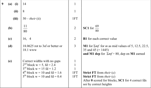
Sam records journey times of 80 people. The cumulative frequency curve gives the results.

(a(i)) Find the median. [1]
(a(ii)) Find the lower quartile. [1]
(a(iii)) Find the interquartile range. [1]
(b) Find, as a fraction, the probability a randomly selected journey took more than 35 minutes. [2]
| Time (min) | \(0<m\le10\) | \(10<m\le15\) | \(15<m\le30\) | \(30<m\le40\) | \(40<m\le50\) |
|---|---|---|---|---|---|
| Frequency | 30 | 12 | 18 | … | … |
(c) Complete the table using the curve. [2]
(d) Estimate the mean using mid-interval values. [3]

(e) Complete the histogram; one column is drawn. [5]

0580 P22 - Nov 2013 - Q20 - 7 marks
48 people visit a museum. The graph records the time each spends there.

(a) Find the median. [1]
(b) Find the 20th percentile. [2]
(c) Find the interquartile range. [2]
(d) Find the probability a random person spends 2 hours or less. [2]

0580 P23 - Nov 2013 - Q18 - 7 marks
A gardener measures 50 green beans. Their lengths are shown by the cumulative frequency graph.

(a) Find the median. [1]
(b) How many beans are longer than 26 cm? [2]
(c) Find the interquartile range. [2]
(d) Find the probability a random bean is more than 14 cm long. [2]

0580 P22 - Jun 2012 - Q15 - 5 marks

The cumulative frequency curve records heights of 60 tomato plants.
(a) Find the median. [1]
(b) Find the lower quartile. [1]
(c) Find the interquartile range. [1]
(d) Find P(height > 15 cm). [2]

0580 P21 - Nov 2012 - Q18 - 6 marks
Lauris records the masses and grades of 300 eggs.
| Mass x (g) | \(30<x\le40\) | \(40<x\le50\) | \(50<x\le60\) | \(60<x\le70\) | \(70<x\le80\) | \(80<x\le90\) |
|---|---|---|---|---|---|---|
| Frequency | 15 | 48 | 72 | 81 | 54 | 30 |
| Grade | small | small | medium | large | very large | very large |
(a) Find the probability that an egg selected at random is very large. [1]
Use the cumulative frequency diagram for part (b).

(b(i)) Find the median mass. [1]
(b(ii)) Find the lower quartile. [1]
(b(iii)) Find the interquartile range. [1]
(b(iv)) Find the number of eggs with mass greater than 65 g. [2]

0580 P43 - Nov 2012 - Q9 - 10 marks
200 students sit a mathematics examination. The diagram records the time t minutes taken to finish.

(a(i)) Find the median. [1]
(a(ii)) Find the lower quartile. [1]
(a(iii)) Find the interquartile range. [1]
(a(iv)) Find how many took more than 1 hour. [2]
| Time t (min) | \(30<t\le40\) | \(40<t\le50\) | \(50<t\le60\) | \(60<t\le70\) | \(70<t\le80\) | \(80<t\le90\) |
|---|---|---|---|---|---|---|
| Frequency | 9 | 16 | 28 | 108 | 28 |
(b(i)) Complete the grouped frequency table using the diagram. [1]
(b(ii)) Estimate the mean completion time, showing working. [4]

0580 P42 - Jun 2011 - Q6 - 19 marks
150 students record their homework completion times.
| Time t (min) | \(0<t\le20\) | \(20<t\le35\) | \(35<t\le45\) | \(45<t\le55\) | \(55<t\le70\) | \(70<t\le80\) |
|---|---|---|---|---|---|---|
| Frequency | 6 | 15 | 19 | 37 | 53 | 20 |
(a)(i) State the interval containing the median. [1]
(a)(ii) Estimate the mean using midpoints 10, 27.5, … . [3]
| Upper time (min) | 20 | 35 | 45 | 55 | 70 | 80 |
|---|---|---|---|---|---|---|
| Cumulative frequency | 6 | 21 |
(b)(i) Complete the cumulative frequencies. [2]

(b)(ii) Label the horizontal axis 0–80 using 1 cm = 5 minutes and the vertical axis 0–150 using 1 cm = 10 students. Draw the cumulative frequency diagram. [5]
(c)(i) Use your graph to estimate the median. [1]
(c)(ii) Estimate the interquartile range. [2]
(c)(iii) Estimate the number with 50 < t ≤ 60. [1]
(c)(iv) Find, as a fraction, the probability a random student took more than 50 minutes. [2]
(c)(v) Find, as a fraction, the probability two students selected without replacement both took more than 50 minutes. [2]


0580 P43 - Jun 2011 - Q6 - 15 marks

The masses of 200 parcels are shown on the cumulative frequency diagram.
(a)(i) Estimate the median mass. [1]
(a)(ii) Estimate the lower quartile. [1]
(a)(iii) Estimate the interquartile range. [1]
(a)(iv) Estimate the number of parcels with mass greater than 3.5 kg. [2]
| Mass m (kg) | \(0<m\le4\) | \(4<m\le6\) | \(6<m\le7\) | \(7<m\le10\) |
|---|---|---|---|---|
| Frequency | 36 | 50 |
(b)(i) Complete the frequency table using the graph. [2]
(b)(ii) Use the table to estimate the mean. [4]
| Mass m (kg) | \(0<m\le4\) | \(4<m\le6\) | \(6<m\le7\) | \(7<m\le10\) |
|---|---|---|---|---|
| Frequency density | 9 | 16.7 |

(b)(iii) Complete the frequency densities and use them to complete the histogram. [4]


0580 P41 - Nov 2011 - Q3 - 15 marks
Heights of 120 girls in a swimming club:
| Height h (m) | \(1.3<h\le1.4\) | \(1.4<h\le1.5\) | \(1.5<h\le1.6\) | \(1.6<h\le1.7\) | \(1.7<h\le1.8\) | \(1.8<h\le1.9\) |
|---|---|---|---|---|---|---|
| Frequency | 4 | 13 | 33 | 45 | 19 | 6 |
(a)(i) State the modal class. [1]
(a)(ii) Estimate the mean height, showing working. [4]
(b)(i) A girl is selected randomly. Find the probability that her height exceeds 1.8 m. [1]
(b)(ii) Find the probability that two girls selected without replacement both have heights at most 1.8 m. [3]
| Upper h (m) | 1.3 | 1.4 | 1.5 | 1.6 | 1.7 | 1.8 | 1.9 |
|---|---|---|---|---|---|---|---|
| Cumulative frequency | 0 | 4 | 17 | 50 | 114 |
(c)(i) Complete the cumulative frequencies. [1]
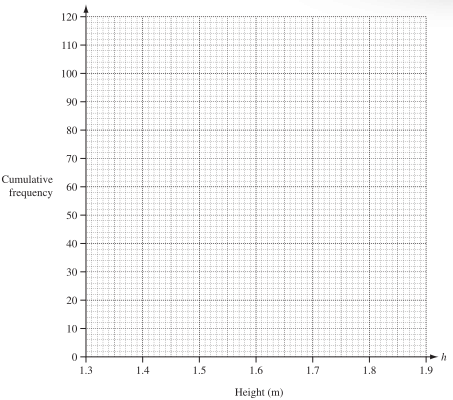
(c)(ii) Draw the cumulative frequency graph. [3]
(d)(i) Use the graph to find the median height. [1]
(d)(ii) Use the graph to find the 30th percentile. [1]


0580 P42 - Nov 2011 - Q5 - 16 marks
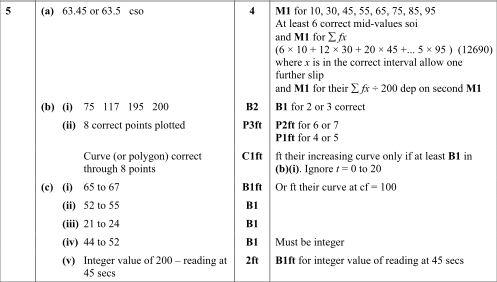
Times for 200 people to solve a problem:
| Time t (s) | \(0<t\le20\) | \(20<t\le40\) | \(40<t\le50\) | \(50<t\le60\) | \(60<t\le70\) | \(70<t\le80\) | \(80<t\le90\) | \(90<t\le100\) |
|---|---|---|---|---|---|---|---|---|
| Frequency | 6 | 12 | 20 | 37 | 42 | 50 | 28 | 5 |
(a) Estimate the mean time. [4]
| Upper time (s) | 20 | 40 | 50 | 60 | 70 | 80 | 90 | 100 |
|---|---|---|---|---|---|---|---|---|
| Cumulative frequency | 6 | 18 | 38 | 167 |
(b)(i) Complete the cumulative frequencies. [2]

(b)(ii) Draw the cumulative frequency graph. [4]
(c)(i) Use the graph to estimate the median. [1]
(c)(ii) Estimate the lower quartile. [1]
(c)(iii) Estimate the interquartile range. [1]
(c)(iv) Estimate the number with times between 65 and 75 s. [1]
(c)(v) Estimate the number taking longer than 45 s. [2]

0580 P43 - Nov 2011 - Q7 - 12 marks
Times for 200 students to cycle one kilometre:
| Time t (min) | \(0<t\le2\) | \(2<t\le3\) | \(3<t\le4\) | \(4<t\le8\) |
|---|---|---|---|---|
| Frequency | 24 | 68 | 72 | 36 |
(a) State the class containing the median. [1]
(b) Estimate the mean with full working. [4]
| Upper time (min) | 2 | 3 | 4 | 8 |
|---|---|---|---|---|
| Cumulative frequency | 24 | 200 |
(c)(i) Complete the cumulative frequencies. [1]

(c)(ii) Draw the cumulative frequency diagram. [3]
(c)(iii) Use it to estimate the median, lower quartile and interquartile range. [3]


0580 P42 - Jun 2010 - Q7 - 15 marks
200 students report weekly exercise time:
| Time t (hours) | \(0<t\le5\) | \(5<t\le10\) | \(10<t\le15\) | \(15<t\le20\) | \(20<t\le25\) | \(25<t\le30\) | \(30<t\le35\) | \(35<t\le40\) |
|---|---|---|---|---|---|---|---|---|
| Frequency | 12 | 15 | 23 | 30 | 40 | 35 | 25 | 20 |
(a) Estimate the mean. [4]
| t ≤ | 5 | 10 | 15 | 20 | 25 | 30 | 35 | 40 |
|---|---|---|---|---|---|---|---|---|
| Cumulative frequency | 12 | 27 | 50 | 80 | 120 | 200 |
(b) Complete the cumulative frequencies. [1]

(c) Draw a cumulative frequency diagram. [4]
(d) Show how to find the lower quartile on the graph. [1]
(e)(i) Estimate the median. [1]
(e)(ii) Estimate the interquartile range. [1]
(e)(iii) Estimate the 64th percentile. [1]
(e)(iv) Estimate the number exercising for more than 17 hours. [2]


0580 P42 - Nov 2010 - Q3 - 11 marks
The masses of 80 boys are shown by the cumulative frequency curve.

(a)(i) Read the median mass. [1]
(a)(ii) Read the lower quartile. [1]
(a)(iii) Read the interquartile range. [1]
(b) How many boys exceed 60 kg? [2]
| Mass m (kg) | Frequency |
|---|---|
| \(30<m\le40\) | 8 |
| \(40<m\le50\) | |
| \(50<m\le60\) | 14 |
| \(60<m\le70\) | 22 |
| \(70<m\le80\) | |
| \(80<m\le90\) | 10 |
(c)(i) Complete the frequencies using the curve. [2]
(c)(ii) Estimate the mean mass. [4]


0580 P41 - Nov 2010 - Q5 - 16 marks
| Height h ≤ (cm) | 130 | 140 | 150 | 160 | 165 | 170 | 180 | 190 |
|---|---|---|---|---|---|---|---|---|
| Cumulative frequency | 0 | 10 | 50 | 95 | 115 | 145 | 180 | 200 |

(a) Draw the cumulative frequency diagram for these 200 students. [4]
(b)(i) Read the median. [1]
(b)(ii) Read the upper quartile. [1]
(b)(iii) Read the interquartile range. [1]
(c)(i) A student is selected randomly. Find the fraction with height greater than 170 cm. [1]
(c)(ii) Select two students without replacement. Find the probability one exceeds 170 cm and the other is 140 cm or shorter. [3]
| Height (cm) | \(130<h\le140\) | \(140<h\le150\) | \(150<h\le160\) | \(160<h\le165\) | \(165<h\le170\) | \(170<h\le180\) | \(180<h\le190\) |
|---|---|---|---|---|---|---|---|
| Frequency | 10 | 40 | 45 | 20 |
(d)(i) Complete the frequency table. [2]

(d)(ii) Complete the histogram. [3]

