Exam-Style Problems
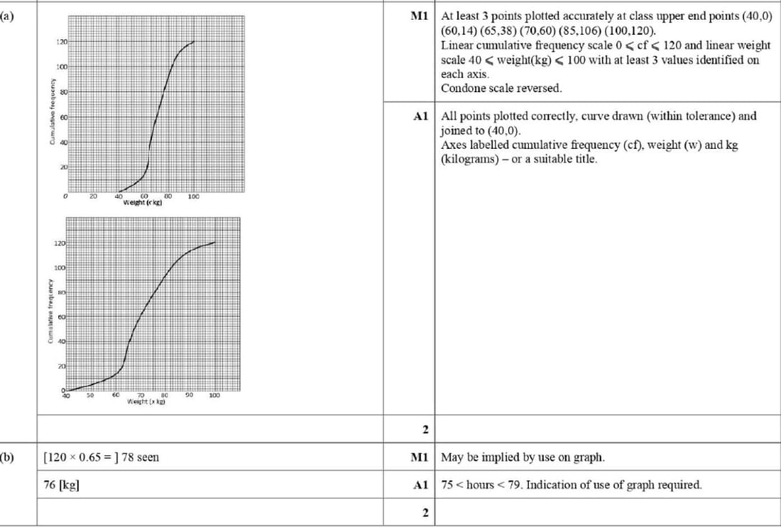
⬅ Back to SubchapterNov 2023 p53 q4
The weights, x kg, of 120 students in a sports college are recorded. The results are summarised in the following table.
| Weight (x kg) | \(x ≤40\) | \(x ≤ 60\) | \(x ≤ 65\) | \(x ≤ 70\) | \(x ≤ 85\) | \(x ≤ 100\) |
|---|---|---|---|---|---|---|
| Cumulative frequency | 0 | 14 | 38 | 60 | 106 | 120 |
(a) Draw a cumulative frequency graph to represent this information.
(b) It is found that 35% of the students weigh more than W kg. Use your graph to estimate the value of W.
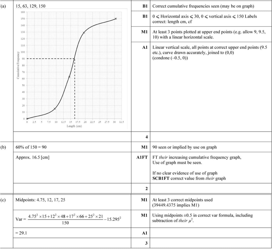
Feb/Mar 2020 p52 q7
Helen measures the lengths of 150 fish of a certain species in a large pond. These lengths, correct to the nearest centimetre, are summarised in the following table.
| Length (cm) | 0 – 9 | 10 – 14 | 15 – 19 | 20 – 30 |
|---|---|---|---|---|
| Frequency | 15 | 48 | 66 | 21 |
(a) Draw a cumulative frequency graph to illustrate the data.
(b) 40% of these fish have a length of d cm or more. Use your graph to estimate the value of d.
The mean length of these 150 fish is 15.295 cm.
(c) Calculate an estimate for the variance of the lengths of the fish.
Nov 2019 p61 q5
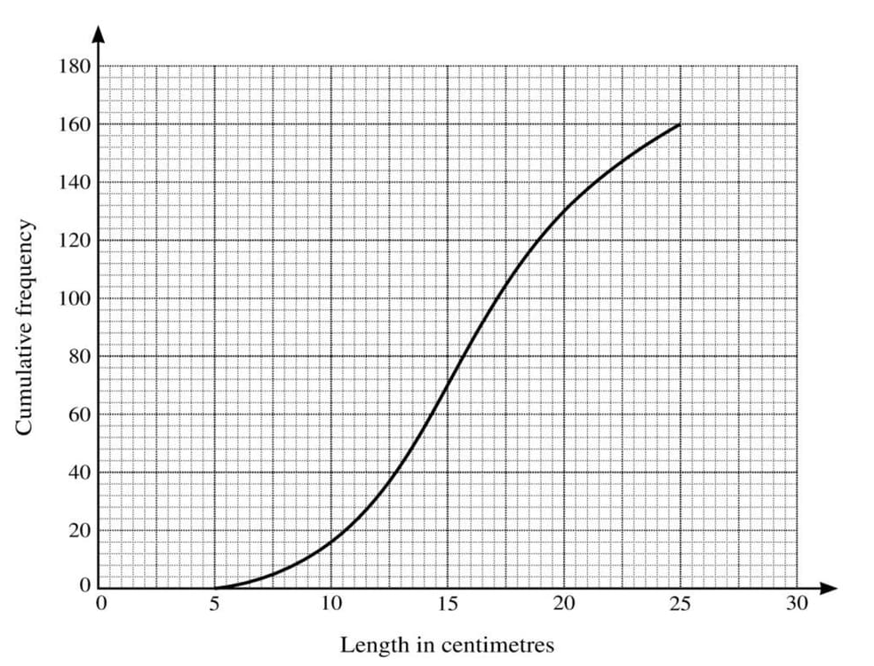
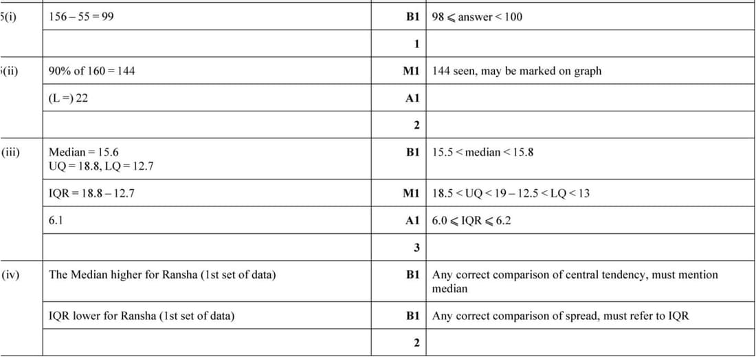
Ransha measured the lengths, in centimetres, of 160 palm leaves. His results are illustrated in the cumulative frequency graph below.
(i) Estimate how many leaves have a length between 14 and 24 centimetres.
(ii) 10% of the leaves have a length of \(L\) centimetres or more. Estimate the value of \(L\).
(iii) Estimate the median and the interquartile range of the lengths.
Sharim measured the lengths, in centimetres, of 160 palm leaves of a different type. He drew a box-and-whisker plot for the data, as shown on the grid below.
(iv) Compare the central tendency and the spread of the two sets of data.
June 2019 p61 q4
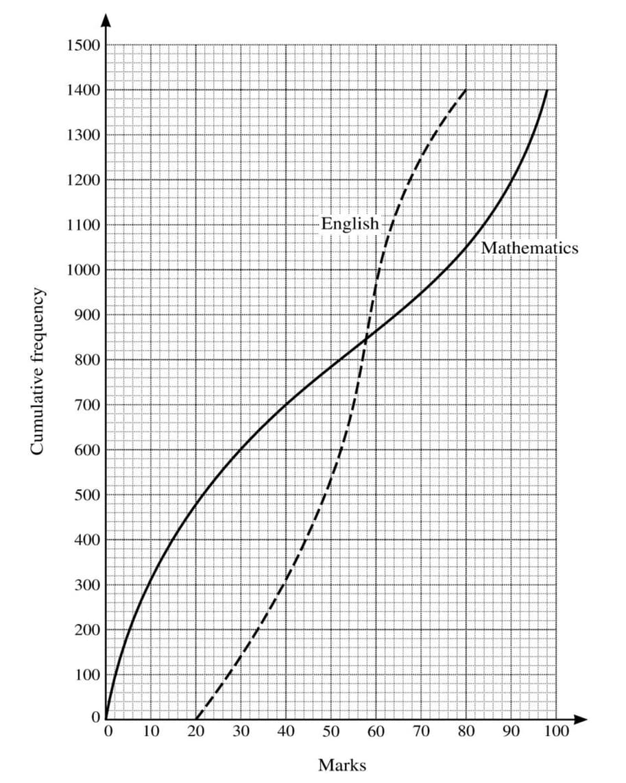
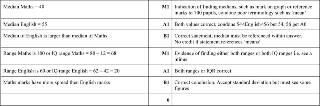
The Mathematics and English A-level marks of 1400 pupils all taking the same examinations are shown in the cumulative frequency graphs below. Both examinations are marked out of 100.
Use suitable data from these graphs to compare the central tendency and spread of the marks in Mathematics and English.
Nov 2019 p63 q5
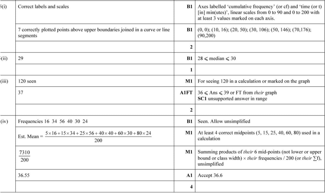
Last Saturday, 200 drivers entering a car park were asked the time, in minutes, that it had taken them to travel from home to the car park. The results are summarised in the following cumulative frequency table.
| Time (t minutes) | \(t \leq 10\) | \(t \leq 20\) | \(t \leq 30\) | \(t \leq 50\) | \(t \leq 70\) | \(t \leq 90\) |
|---|---|---|---|---|---|---|
| Cumulative frequency | 16 | 50 | 106 | 146 | 176 | 200 |
- On the grid, draw a cumulative frequency graph to illustrate the data. [2]
- Use your graph to estimate the median of the data. [1]
- For 80 of the drivers, the time taken was at least \(T\) minutes. Use your graph to estimate the value of \(T\). [2]
- Calculate an estimate of the mean time taken by all 200 drivers to travel to the car park. [4]
Nov 2018 p61 q6
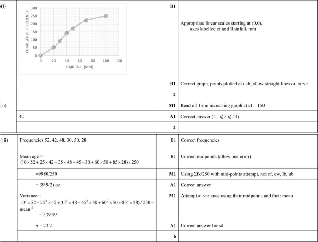
The daily rainfall, \(x\) mm, in a certain village is recorded on 250 consecutive days. The results are summarised in the following cumulative frequency table.
| Rainfall, \(x\) mm | \(x \leq 20\) | \(x \leq 30\) | \(x \leq 40\) | \(x \leq 50\) | \(x \leq 70\) | \(x \leq 100\) |
|---|---|---|---|---|---|---|
| Cumulative frequency | 52 | 94 | 142 | 172 | 222 | 250 |
- On the grid, draw a cumulative frequency graph to illustrate the data. [2]
- On 100 of the days, the rainfall was \(k\) mm or more. Use your graph to estimate the value of \(k\). [2]
- Calculate estimates of the mean and standard deviation of the daily rainfall in this village. [6]
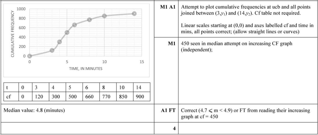
Feb/Mar 2018 p62 q1
There are 900 students in a certain year-group. An identical puzzle is given to each student and the time taken, \(t\) minutes, to complete the puzzle is recorded. These times are summarised in the following frequency table.
| Time taken, \(t\) minutes | \(t \leq 3\) | \(3 < t \leq 4\) | \(4 < t \leq 5\) | \(5 < t \leq 6\) | \(6 < t \leq 8\) | \(8 < t \leq 10\) | \(10 < t \leq 14\) |
|---|---|---|---|---|---|---|---|
| Frequency | 120 | 180 | 200 | 160 | 110 | 80 | 50 |
On the grid, draw a cumulative frequency graph to represent the data. Use your graph to estimate the median time taken by these students to complete the puzzle.
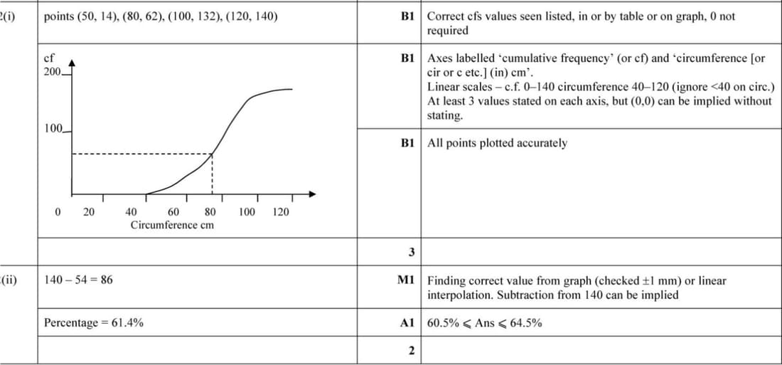
Nov 2017 p62 q2
The circumferences, \(c\) cm, of some trees in a wood were measured. The results are summarised in the table.
| Circumference (c cm) | \(40 < c \leq 50\) | \(50 < c \leq 80\) | \(80 < c \leq 100\) | \(100 < c \leq 120\) |
|---|---|---|---|---|
| Frequency | 14 | 48 | 70 | 8 |
(i) On the grid, draw a cumulative frequency graph to represent the information.
(ii) Estimate the percentage of trees which have a circumference larger than 75 cm.
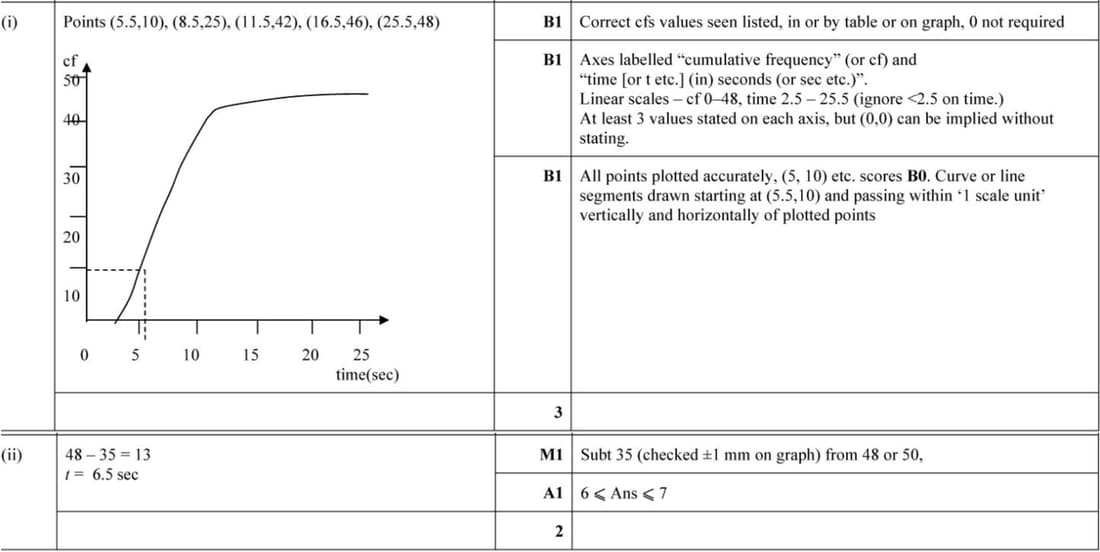
Nov 2017 p61 q2
The time taken by a car to accelerate from 0 to 30 metres per second was measured correct to the nearest second. The results from 48 cars are summarised in the following table.
| Time (seconds) | 3 – 5 | 6 – 8 | 9 – 11 | 12 – 16 | 17 – 25 |
|---|---|---|---|---|---|
| Frequency | 10 | 15 | 17 | 4 | 2 |
(i) On the grid, draw a cumulative frequency graph to represent this information. [3]
(ii) 35 of these cars accelerated from 0 to 30 metres per second in a time more than \(t\) seconds. Estimate the value of \(t\). [2]
June 2017 p63 q7
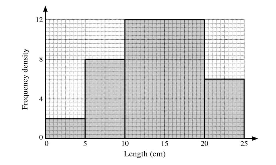
The following histogram represents the lengths of worms in a garden.
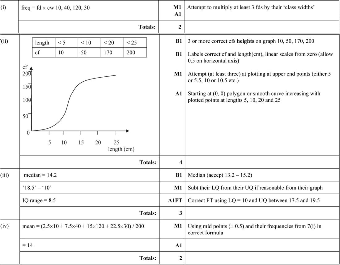
(i) Calculate the frequencies represented by each of the four histogram columns.
(ii) On the grid on the next page, draw a cumulative frequency graph to represent the lengths of worms in the garden.
(iii) Use your graph to estimate the median and interquartile range of the lengths of worms in the garden.
(iv) Calculate an estimate of the mean length of worms in the garden.
June 2017 p62 q2
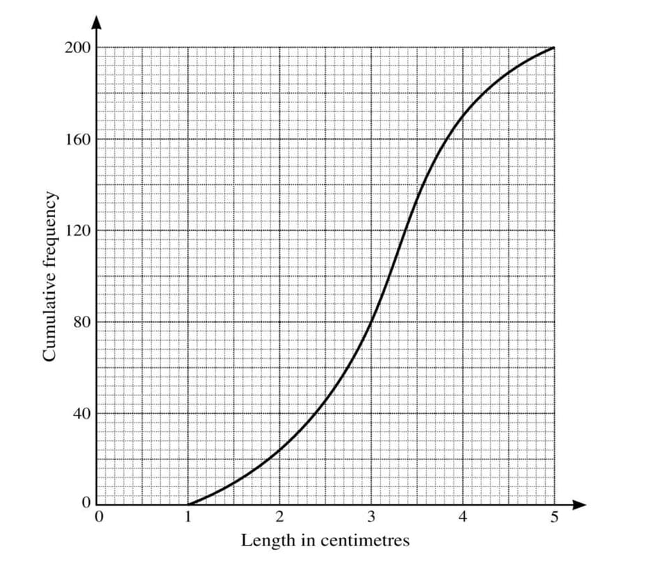
Anabel measured the lengths, in centimetres, of 200 caterpillars. Her results are illustrated in the cumulative frequency graph below.
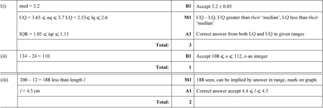
(i) Estimate the median and the interquartile range of the lengths.
(ii) Estimate how many caterpillars had a length of between 2 and 3.5 cm.
(iii) 6% of caterpillars were of length \(l\) centimetres or more. Estimate \(l\).
Nov 2023 p51 q1
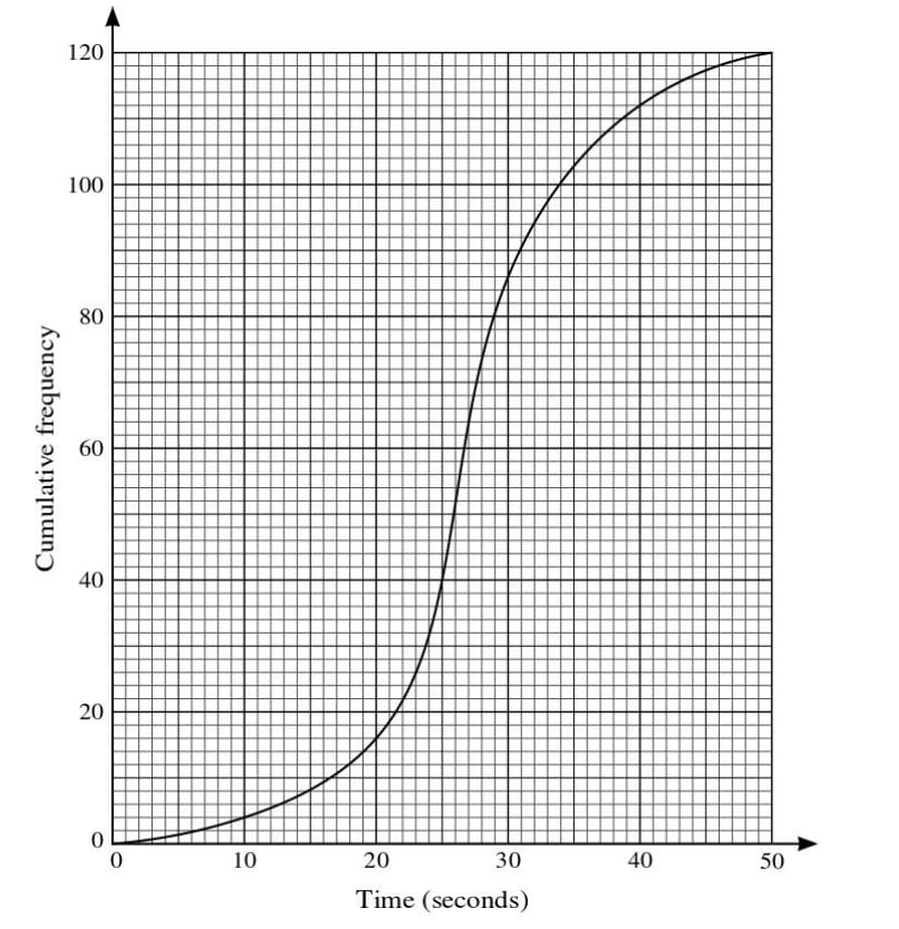
The times taken by 120 children to complete a particular puzzle are represented in the cumulative frequency graph.
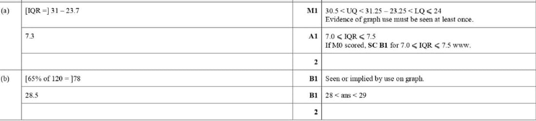
(a) Use the graph to estimate the interquartile range of the data.
35% of the children took longer than \(T\) seconds to complete the puzzle.
(b) Use the graph to estimate the value of \(T\).
Nov 2016 p63 q5
The tables summarise the heights, \(h\) (cm), of 60 girls and 60 boys.
| Height of girls (cm) | \(140 < h \le 150\) | \(150 < h \le 160\) | \(160 < h \le 170\) | \(170 < h \le 180\) | \(180 < h \le 190\) |
|---|---|---|---|---|---|
| Frequency | 12 | 21 | 17 | 10 | 0 |
| Height of boys (cm) | \(140 < h \le 150\) | \(150 < h \le 160\) | \(160 < h \le 170\) | \(170 < h \le 180\) | \(180 < h \le 190\) |
|---|---|---|---|---|---|
| Frequency | 0 | 20 | 23 | 12 | 5 |
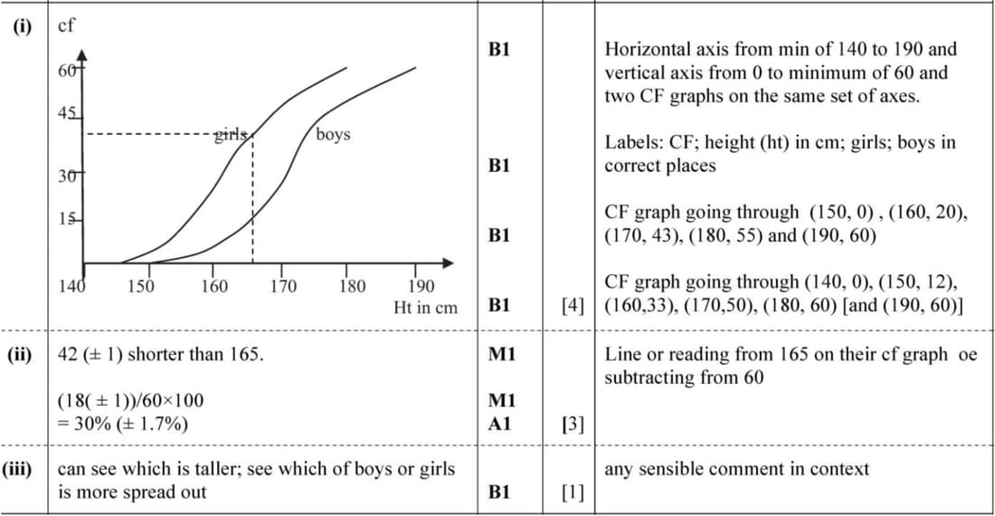
- On graph paper, using the same axes, draw two cumulative frequency graphs to illustrate the data.
- The cave on the school trip is \(165\ \text{cm}\) high. Use your graph to estimate the percentage of girls who will be unable to stand upright.
- State one advantage of using a pair of box-and-whisker plots rather than cumulative frequency graphs to compare the heights of the girls and the boys.
June 2016 p61 q7
The amounts spent by 160 shoppers at a supermarket are summarised in the following table.
| Amount spent \((x)\) | \(0 < x \le 30\) | \(30 < x \le 50\) | \(50 < x \le 70\) | \(70 < x \le 90\) | \(90 < x \le 140\) |
|---|---|---|---|---|---|
| Number of shoppers | 16 | 40 | 48 | 26 | 30 |
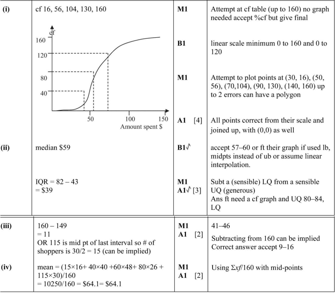
- Draw a cumulative frequency graph of this distribution.
- Estimate the median and the interquartile range of the amount spent.
- Estimate the number of shoppers who spent more than \(\$115\).
- Calculate an estimate of the mean amount spent.
June 2015 p63 q6
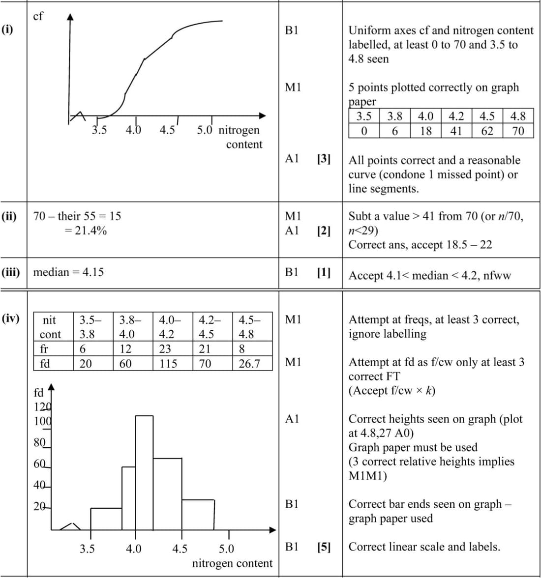
Seventy samples of fertiliser were collected and the nitrogen content was measured for each sample. The cumulative frequency distribution is shown below.
| Nitrogen content | \(\le 3.5\) | \(\le 3.8\) | \(\le 4.0\) | \(\le 4.2\) | \(\le 4.5\) | \(\le 4.8\) |
|---|---|---|---|---|---|---|
| Cumulative frequency | 0 | 6 | 18 | 41 | 62 | 70 |
- On graph paper, draw a cumulative frequency graph to represent the data.
- Estimate the percentage of samples with a nitrogen content greater than \(4.4\).
- Estimate the median.
- Construct a frequency table for these results and draw a histogram on graph paper.
June 2015 p62 q3
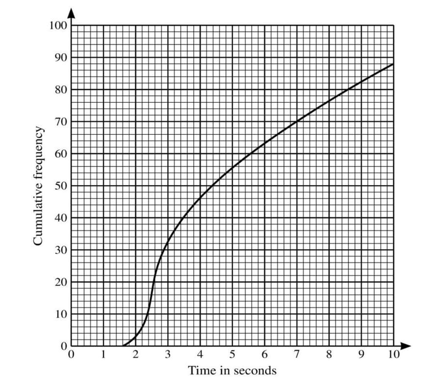
In an open-plan office there are 88 computers. The times taken by these 88 computers to access a particular web page are represented in the cumulative frequency diagram.
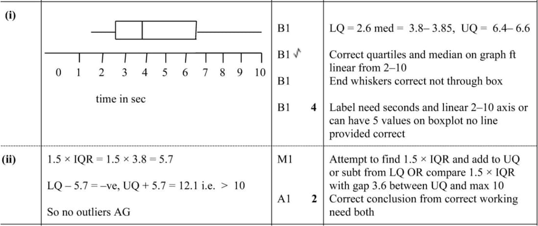
(i) On graph paper draw a box-and-whisker plot to summarise this information.An ‘outlier’ is defined as any data value which is more than 1.5 times the interquartile range above the upper quartile, or more than 1.5 times the interquartile range below the lower quartile.
(ii) Show that there are no outliers.
Nov 2014 p62 q6
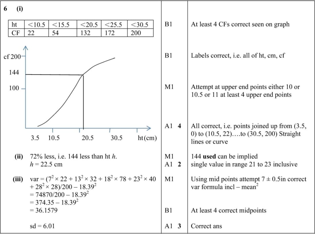
On a certain day in spring, the heights of 200 daffodils are measured, correct to the nearest centimetre. The frequency distribution is given below.
| Height (cm) | 4 – 10 | 11 – 15 | 16 – 20 | 21 – 25 | 26 – 30 |
|---|---|---|---|---|---|
| Frequency | 22 | 32 | 78 | 40 | 28 |
- Draw a cumulative frequency graph to illustrate the data.
- 28% of these daffodils are of height h cm or more. Estimate h.
- You are given that the estimate of the mean height of these daffodils, calculated from the table, is 18.39 cm. Calculate an estimate of the standard deviation of the heights of these daffodils.
June 2013 p63 q6
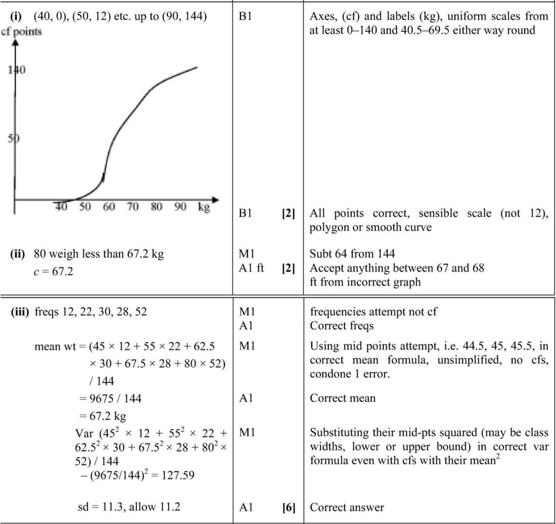
The weights, \(x\) kilograms, of 144 people were recorded. The results are summarised in the cumulative frequency table below.
| Weight (\(x\) kilograms) | \(x < 40\) | \(x < 50\) | \(x < 60\) | \(x < 65\) | \(x < 70\) | \(x < 90\) |
|---|---|---|---|---|---|---|
| Cumulative frequency | 0 | 12 | 34 | 64 | 92 | 144 |
- On graph paper, draw a cumulative frequency graph to represent these results.
- 64 people weigh more than \(c\) kg. Use your graph to find the value of \(c\).
- Calculate estimates of the mean and standard deviation of the weights.
Nov 2011 p63 q5
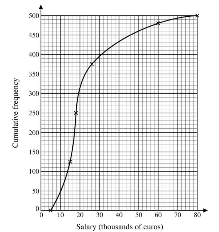
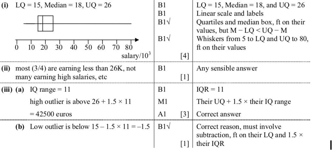
The cumulative frequency graph shows the annual salaries, in thousands of euros, of a random sample of 500 adults with jobs, in France. It has been plotted using grouped data. You may assume that the lowest salary is 5000 euros and the highest salary is 80000 euros.
- On graph paper, draw a box-and-whisker plot to illustrate these salaries.
- Comment on the salaries of the people in this sample.
- An ‘outlier’ is defined as any data value which is more than 1.5 times the interquartile range above the upper quartile, or more than 1.5 times the interquartile range below the lower quartile.
- How high must a salary be in order to be classified as an outlier?
- Show that none of the salaries is low enough to be classified as an outlier.
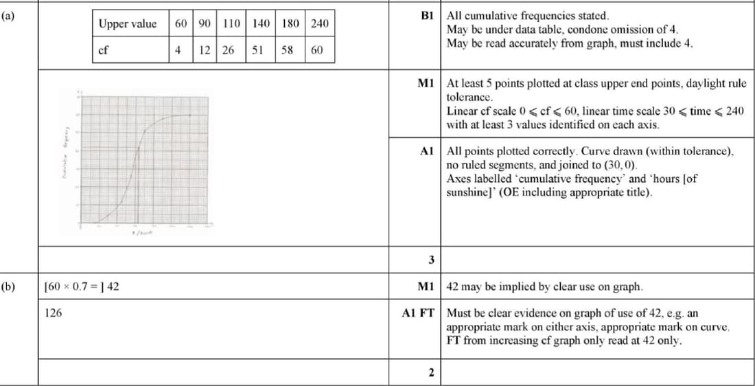
June 2011 p63 q3
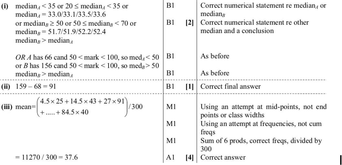
The following cumulative frequency table shows the examination marks for 300 candidates in country A and 300 candidates in country B.
| Mark | \(< 10\) | \(< 20\) | \(< 35\) | \(< 50\) | \(< 70\) | \(< 100\) |
|---|---|---|---|---|---|---|
| Cumulative frequency, A | 25 | 68 | 159 | 234 | 260 | 300 |
| Cumulative frequency, B | 10 | 46 | 72 | 144 | 198 | 300 |
- Without drawing a graph, show that the median for country B is higher than the median for country A.
- Find the number of candidates in country A who scored between 20 and 34 marks inclusive.
- Calculate an estimate of the mean mark for candidates in country A.
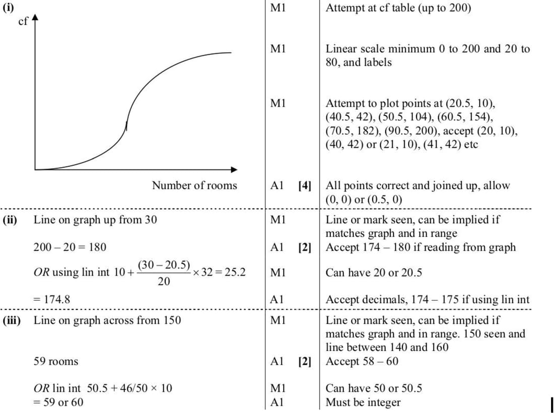
June 2011 p62 q5
A hotel has 90 rooms. The table summarises information about the number of rooms occupied each day for a period of 200 days.
| Number of rooms occupied | 1 – 20 | 21 – 40 | 41 – 50 | 51 – 60 | 61 – 70 | 71 – 90 |
|---|---|---|---|---|---|---|
| Frequency | 10 | 32 | 62 | 50 | 28 | 18 |
- Draw a cumulative frequency graph on graph paper to illustrate this information.
- Estimate the number of days when over 30 rooms were occupied.
- On 75% of the days at most n rooms were occupied. Estimate the value of n.
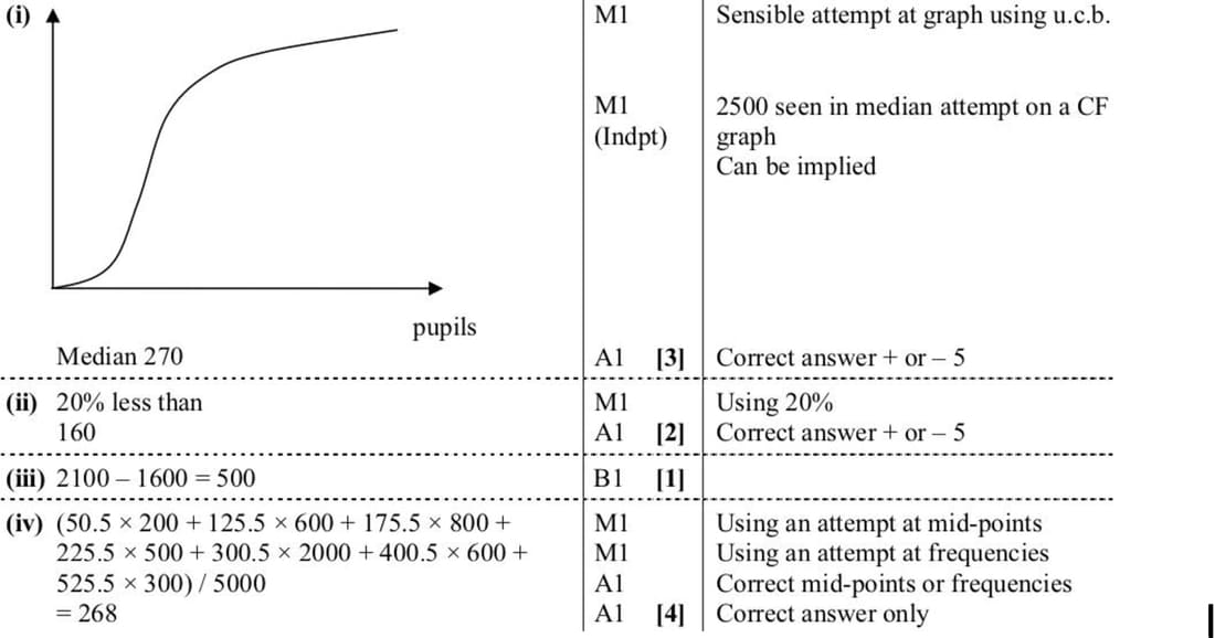
June 2011 p61 q6
There are 5000 schools in a certain country. The cumulative frequency table shows the number of pupils in a school and the corresponding number of schools.
| Number of pupils in a school | \(\leq 100\) | \(\leq 150\) | \(\leq 200\) | \(\leq 250\) | \(\leq 350\) | \(\leq 450\) | \(\leq 600\) |
|---|---|---|---|---|---|---|---|
| Cumulative frequency | 200 | 800 | 1600 | 2100 | 4100 | 4700 | 5000 |
- Draw a cumulative frequency graph with a scale of 2 cm to 100 pupils on the horizontal axis and a scale of 2 cm to 1000 schools on the vertical axis. Use your graph to estimate the median number of pupils in a school.
- 80% of the schools have more than \(n\) pupils. Estimate the value of \(n\) correct to the nearest ten.
- Find how many schools have between 201 and 250 (inclusive) pupils.
- Calculate an estimate of the mean number of pupils per school.
Feb/Mar 2023 p52 q1
Each year the total number of hours, \(x\), of sunshine in Kintoo is recorded during the month of June. The results for the last 60 years are summarised in the table.
| \(x\) | 30 \(\leq x <\) 60 | 60 \(\leq x <\) 90 | 90 \(\leq x <\) 110 | 110 \(\leq x <\) 140 | 140 \(\leq x <\) 180 | 180 \(\leq x <\) 240 |
|---|---|---|---|---|---|---|
| Number of years | 4 | 8 | 14 | 25 | 7 | 2 |
(a) Draw a cumulative frequency graph to illustrate the data.
(b) Use your graph to estimate the 70th percentile of the data.
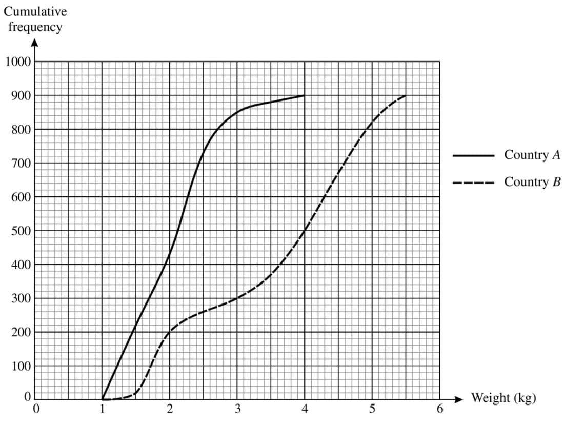
June 2010 p62 q3
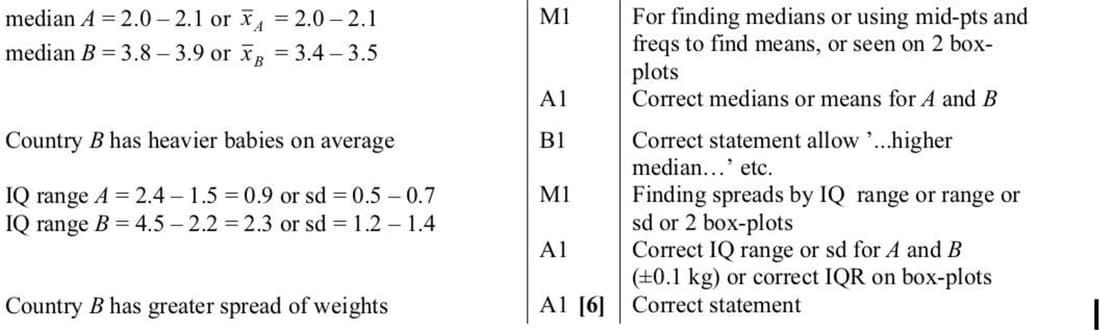
The birth weights of random samples of 900 babies born in country A and 900 babies born in country B are illustrated in the cumulative frequency graphs. Use suitable data from these graphs to compare the central tendency and spread of the birth weights of the two sets of babies.
June 2009 p6 q6
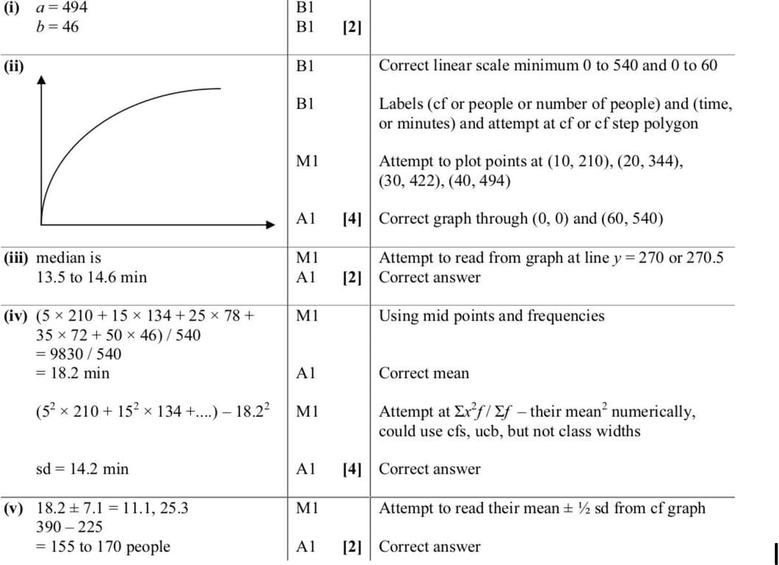
During January the numbers of people entering a store during the first hour after opening were as follows.
| Time after opening, x minutes | Frequency | Cumulative frequency |
|---|---|---|
| 0 < x ≤ 10 | 210 | 210 |
| 10 < x ≤ 20 | 134 | 344 |
| 20 < x ≤ 30 | 78 | 422 |
| 30 < x ≤ 40 | 72 | a |
| 40 < x ≤ 60 | b | 540 |
- Find the values of a and b.
- Draw a cumulative frequency graph to represent this information. Take a scale of 2 cm for 10 minutes on the horizontal axis and 2 cm for 50 people on the vertical axis.
- Use your graph to estimate the median time after opening that people entered the store.
- Calculate estimates of the mean, m minutes, and standard deviation, s minutes, of the time after opening that people entered the store.
- Use your graph to estimate the number of people entering the store between \(m - \frac{1}{2}s\) and \(m + \frac{1}{2}s\) minutes after opening.
Nov 2007 p6 q5
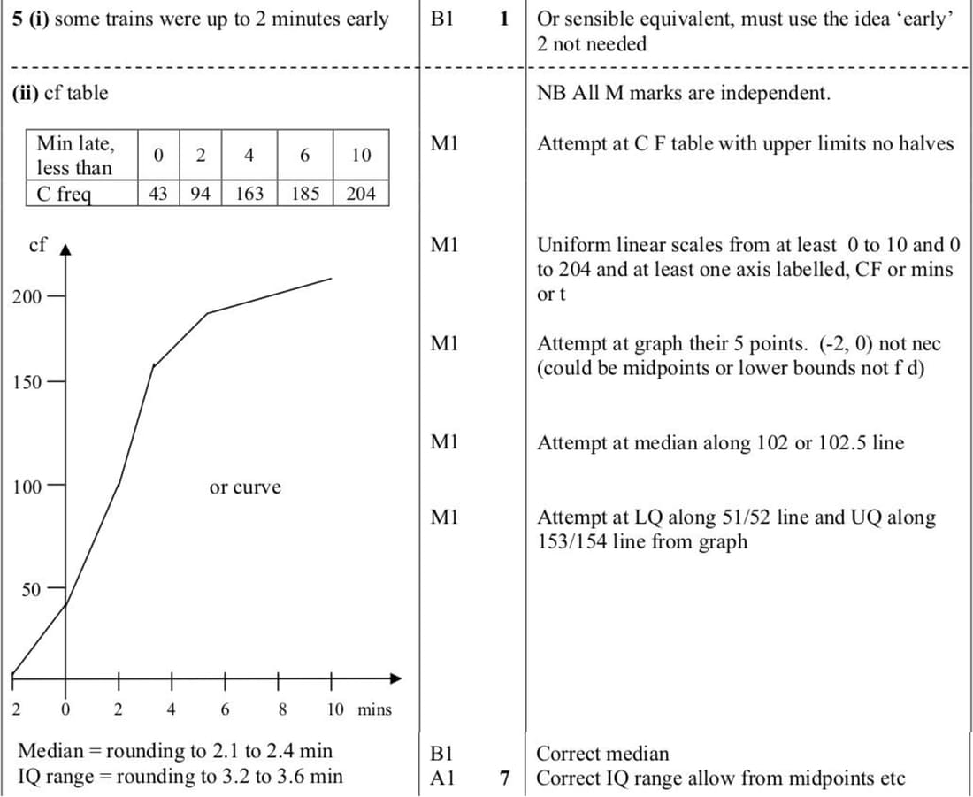
The arrival times of 204 trains were noted and the number of minutes, t, that each train was late was recorded. The results are summarised in the table.
| Number of minutes late (t) | -2 ≤ t < 0 | 0 ≤ t < 2 | 2 ≤ t < 4 | 4 ≤ t < 6 | 6 ≤ t < 10 |
|---|---|---|---|---|---|
| Number of trains | 43 | 51 | 69 | 22 | 19 |
- Explain what -2 ≤ t < 0 means about the arrival times of trains.
- Draw a cumulative frequency graph, and from it estimate the median and the interquartile range of the number of minutes late of these trains.
June 2004 p6 q2
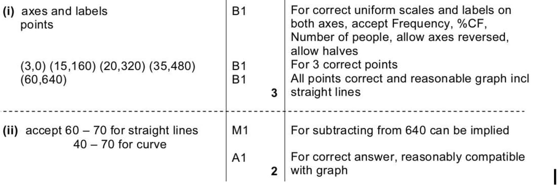
In a recent survey, 640 people were asked about the length of time each week that they spent watching television. The median time was found to be 20 hours, and the lower and upper quartiles were 15 hours and 35 hours respectively. The least amount of time that anyone spent was 3 hours, and the greatest amount was 60 hours.
- On graph paper, show these results using a fully labelled cumulative frequency graph.
- Use your graph to estimate how many people watched more than 50 hours of television each week.
June 2002 p6 q2
The manager of a company noted the times spent in 80 meetings. The results were as follows.
| Time \((t)\) minutes | \( 0 < t \le 15 \) | \( 15 < t \le 30 \) | \( 30 < t \le 60 \) | \( 60 < t \le 90 \) | \( 90 < t \le 120 \) |
|---|---|---|---|---|---|
| Number of meetings | 4 | 7 | 24 | 38 | 7 |
Draw a cumulative frequency graph and use this to estimate the median time and the interquartile range.
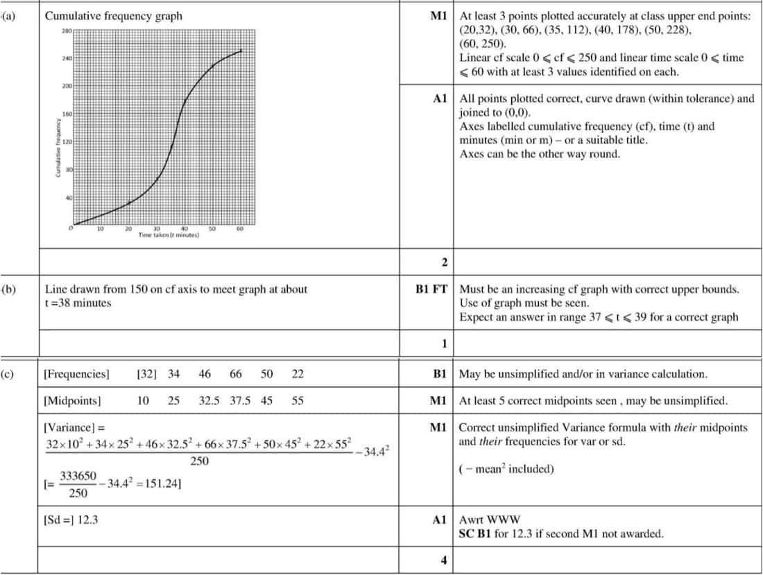
Nov 2022 p53 q3
The times, t minutes, taken to complete a walking challenge by 250 members of a club are summarised in the table.
| Time taken (t minutes) | t ≤ 20 | t ≤ 30 | t ≤ 35 | t ≤ 40 | t ≤ 50 | t ≤ 60 |
|---|---|---|---|---|---|---|
| Cumulative frequency | 32 | 66 | 112 | 178 | 228 | 250 |
(a) Draw a cumulative frequency graph to illustrate the data.
(b) Use your graph to estimate the 60th percentile of the data.
It is given that an estimate for the mean time taken to complete the challenge by these 250 members is 34.4 minutes.
(c) Calculate an estimate for the standard deviation of the times taken to complete the challenge by these 250 members.
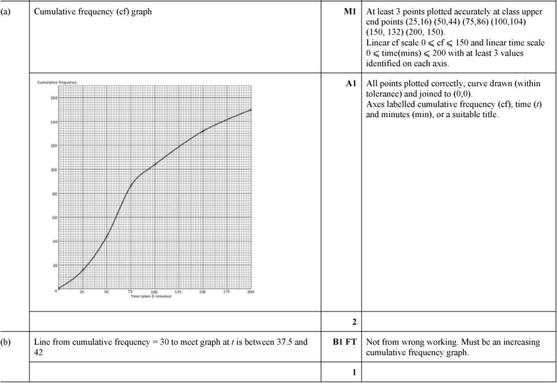
June 2022 p53 q1
The time taken, \(t\) minutes, to complete a puzzle was recorded for each of 150 students. These times are summarised in the table.
| Time taken \((t)\) minutes | \(t \le 25\) | \(t \le 50\) | \(t \le 75\) | \(t \le 100\) | \(t \le 150\) | \(t \le 200\) |
|---|---|---|---|---|---|---|
| Cumulative frequency | 16 | 44 | 86 | 104 | 132 | 150 |
- Draw a cumulative frequency graph to illustrate the data.
- Use your graph to estimate the 20th percentile of the data.
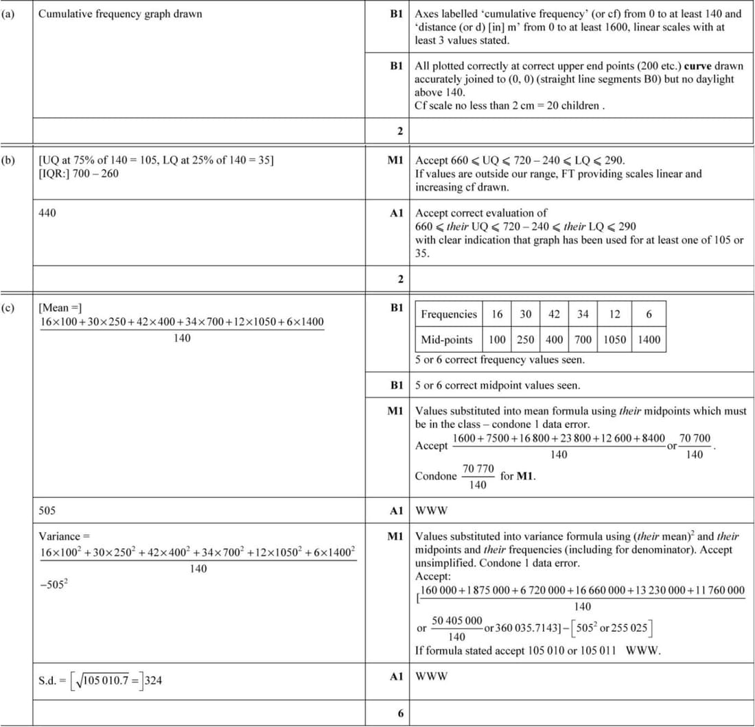
Nov 2021 p52 q7
The distances, x m, travelled to school by 140 children were recorded. The results are summarised in the table below.
| Distance, x m | x ≤ 200 | x ≤ 300 | x ≤ 500 | x ≤ 900 | x ≤ 1200 | x ≤ 1600 |
|---|---|---|---|---|---|---|
| Cumulative frequency | 16 | 46 | 88 | 122 | 134 | 140 |
(a) On the grid, draw a cumulative frequency graph to represent these results.
(b) Use your graph to estimate the interquartile range of the distances.
(c) Calculate estimates of the mean and standard deviation of the distances.
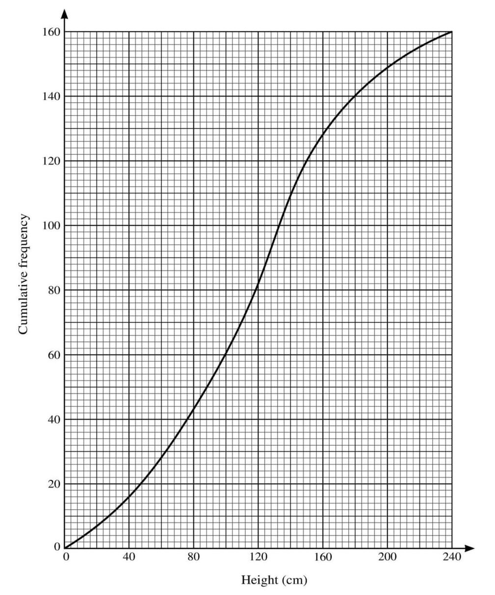
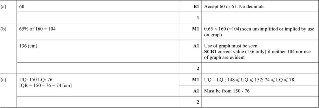
June 2021 p53 q1
The heights in cm of 160 sunflower plants were measured. The results are summarised on the following cumulative frequency curve.
(a) Use the graph to estimate the number of plants with heights less than 100 cm.
(b) Use the graph to estimate the 65th percentile of the distribution.
(c) Use the graph to estimate the interquartile range of the heights of these plants.
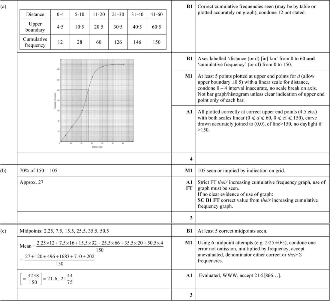
Feb/Mar 2021 p52 q5
A driver records the distance travelled in each of 150 journeys. These distances, correct to the nearest km, are summarised in the following table.
| Distance (km) | 0 – 4 | 5 – 10 | 11 – 20 | 21 – 30 | 31 – 40 | 41 – 60 |
|---|---|---|---|---|---|---|
| Frequency | 12 | 16 | 32 | 66 | 20 | 4 |
(a) Draw a cumulative frequency graph to illustrate the data.
(b) For 30% of these journeys the distance travelled is \(d\) km or more. Use your graph to estimate the value of \(d\).
(c) Calculate an estimate of the mean distance travelled for the 150 journeys.