Exam-Style Problems
⬅ Back to SubchapterNov 2016 p62 q5
2393
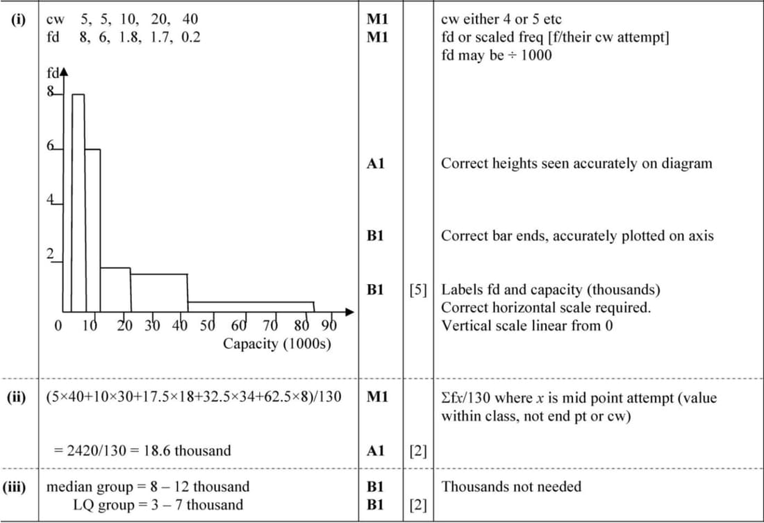
The number of people a football stadium can hold is called the 'capacity'. The capacities of 130 football stadiums in the UK, to the nearest thousand, are summarised in the table.
| Capacity (people) | 3,000–7,000 | 8,000–12,000 | 13,000–22,000 | 23,000–42,000 | 43,000–82,000 |
|---|---|---|---|---|---|
| Number of stadiums | 40 | 30 | 18 | 34 | 8 |
- On graph paper, draw a histogram to represent this information. Use a scale of 2 cm for a capacity of 10,000 on the horizontal axis.
- Calculate an estimate of the mean capacity of these 130 stadiums.
- Find which class in the table contains the median and which contains the lower quartile.
Feb/Mar 2016 p62 q4
2394
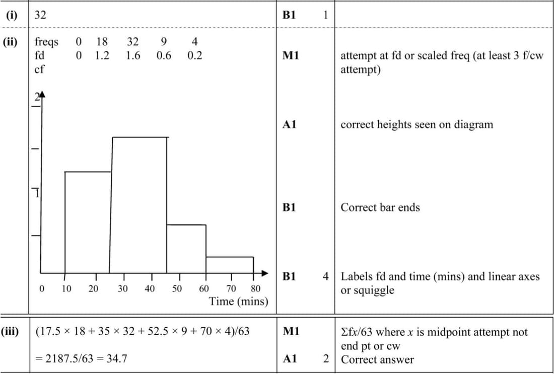
A survey was made of the journey times of 63 people who cycle to work in a certain town. The results are summarised in the following cumulative frequency table.
| Journey time (minutes) | ≤ 10 | ≤ 25 | ≤ 45 | ≤ 60 | ≤ 80 |
|---|---|---|---|---|---|
| Cumulative frequency | 0 | 18 | 50 | 59 | 63 |
- State how many journey times were between 25 and 45 minutes.
- Draw a histogram on graph paper to represent the data.
- Calculate an estimate of the mean journey time.
Nov 2015 p63 q6
2395
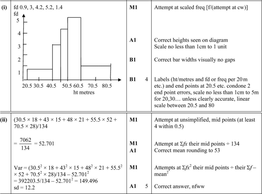
The heights to the nearest metre of 134 office buildings in a certain city are summarised in the table below.
| Height (m) | 21–40 | 41–45 | 46–50 | 51–60 | 61–80 |
|---|---|---|---|---|---|
| Frequency | 18 | 15 | 21 | 52 | 28 |
(i) Draw a histogram on graph paper to illustrate the data.
(ii) Calculate estimates of the mean and standard deviation of these heights.
Nov 2015 p61 q3
2396
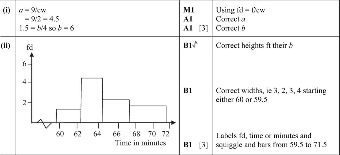
Robert has a part-time job delivering newspapers. On a number of days he noted the time, correct to the nearest minute, that it took him to do his job. Robert used his results to draw up the following table; two of the values in the table are denoted by \(a\) and \(b\).
\(\begin{array}{|c|c|c|c|c|} \hline \text{Time (t minutes)} & 60 - 62 & 63 - 64 & 65 - 67 & 68 - 71 \\ \hline \text{Frequency (number of days)} & 3 & 9 & 6 & b \\ \hline \text{Frequency density} & 1 & a & 2 & 1.5 \\ \hline \end{array}\)
(i) Find the values of \(a\) and \(b\).
(ii) On graph paper, draw a histogram to represent Robert’s times.
June 2015 p61 q2
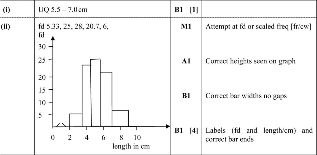
2397
The table summarises the lengths in centimetres of 104 dragonflies.
| Length (cm) | 2.0–3.5 | 3.5–4.5 | 4.5–5.5 | 5.5–7.0 | 7.0–9.0 |
|---|---|---|---|---|---|
| Frequency | 8 | 25 | 28 | 31 | 12 |
- State which class contains the upper quartile.
- Draw a histogram, on graph paper, to represent the data.