Exam-Style Problems
⬅ Back to SubchapterNov 2021 p52 q7
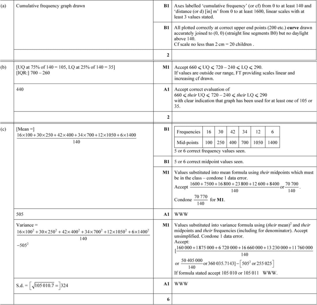
The distances, x m, travelled to school by 140 children were recorded. The results are summarised in the table below.
| Distance, x m | x ≤ 200 | x ≤ 300 | x ≤ 500 | x ≤ 900 | x ≤ 1200 | x ≤ 1600 |
|---|---|---|---|---|---|---|
| Cumulative frequency | 16 | 46 | 88 | 122 | 134 | 140 |
(a) On the grid, draw a cumulative frequency graph to represent these results.
(b) Use your graph to estimate the interquartile range of the distances.
(c) Calculate estimates of the mean and standard deviation of the distances.
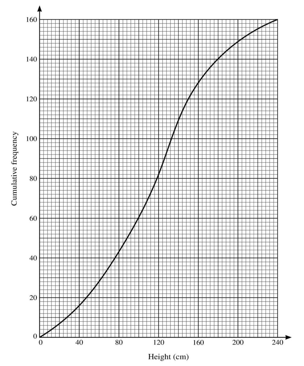
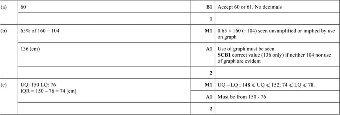
June 2021 p53 q1
The heights in cm of 160 sunflower plants were measured. The results are summarised on the following cumulative frequency curve.
(a) Use the graph to estimate the number of plants with heights less than 100 cm.
(b) Use the graph to estimate the 65th percentile of the distribution.
(c) Use the graph to estimate the interquartile range of the heights of these plants.
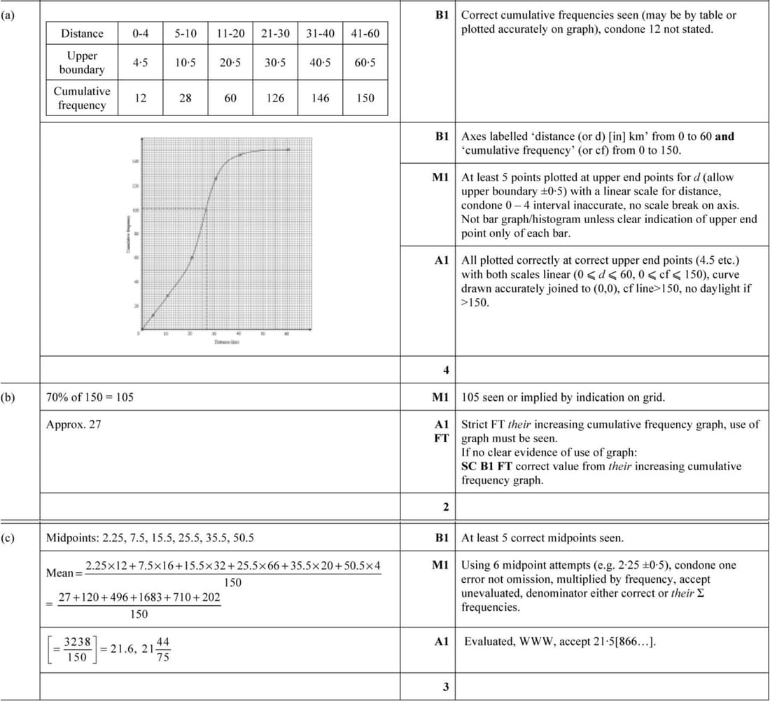
Feb/Mar 2021 p52 q5
A driver records the distance travelled in each of 150 journeys. These distances, correct to the nearest km, are summarised in the following table.
| Distance (km) | 0 – 4 | 5 – 10 | 11 – 20 | 21 – 30 | 31 – 40 | 41 – 60 |
|---|---|---|---|---|---|---|
| Frequency | 12 | 16 | 32 | 66 | 20 | 4 |
(a) Draw a cumulative frequency graph to illustrate the data.
(b) For 30% of these journeys the distance travelled is \(d\) km or more. Use your graph to estimate the value of \(d\).
(c) Calculate an estimate of the mean distance travelled for the 150 journeys.