Exam-Style Problems
⬅ Back to SubchapterJune 2015 p62 q3
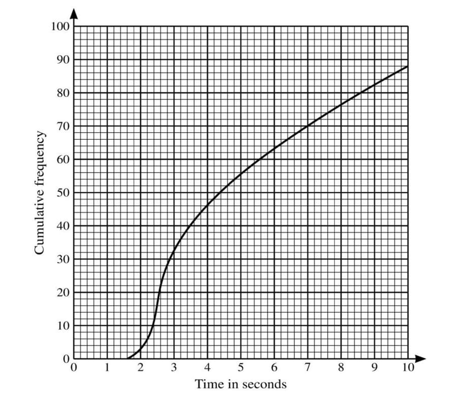
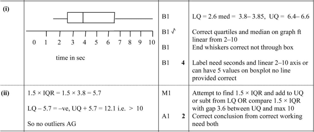
In an open-plan office there are 88 computers. The times taken by these 88 computers to access a particular web page are represented in the cumulative frequency diagram.
(i) On graph paper draw a box-and-whisker plot to summarise this information.An ‘outlier’ is defined as any data value which is more than 1.5 times the interquartile range above the upper quartile, or more than 1.5 times the interquartile range below the lower quartile.
(ii) Show that there are no outliers.
Nov 2014 p62 q6
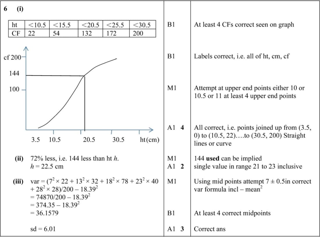
On a certain day in spring, the heights of 200 daffodils are measured, correct to the nearest centimetre. The frequency distribution is given below.
| Height (cm) | 4 – 10 | 11 – 15 | 16 – 20 | 21 – 25 | 26 – 30 |
|---|---|---|---|---|---|
| Frequency | 22 | 32 | 78 | 40 | 28 |
- Draw a cumulative frequency graph to illustrate the data.
- 28% of these daffodils are of height h cm or more. Estimate h.
- You are given that the estimate of the mean height of these daffodils, calculated from the table, is 18.39 cm. Calculate an estimate of the standard deviation of the heights of these daffodils.
June 2013 p63 q6
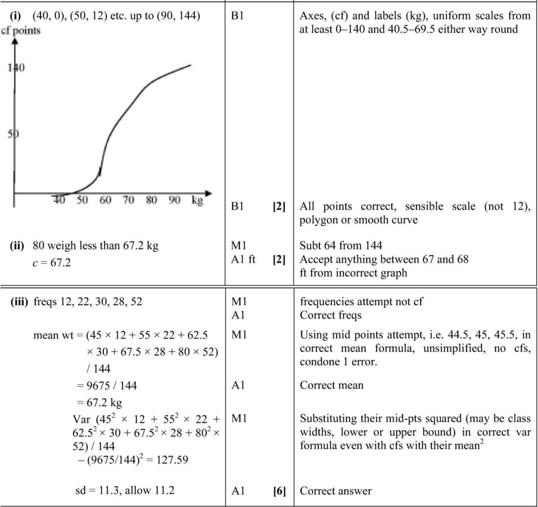
The weights, \(x\) kilograms, of 144 people were recorded. The results are summarised in the cumulative frequency table below.
| Weight (\(x\) kilograms) | \(x < 40\) | \(x < 50\) | \(x < 60\) | \(x < 65\) | \(x < 70\) | \(x < 90\) |
|---|---|---|---|---|---|---|
| Cumulative frequency | 0 | 12 | 34 | 64 | 92 | 144 |
- On graph paper, draw a cumulative frequency graph to represent these results.
- 64 people weigh more than \(c\) kg. Use your graph to find the value of \(c\).
- Calculate estimates of the mean and standard deviation of the weights.
Nov 2011 p63 q5
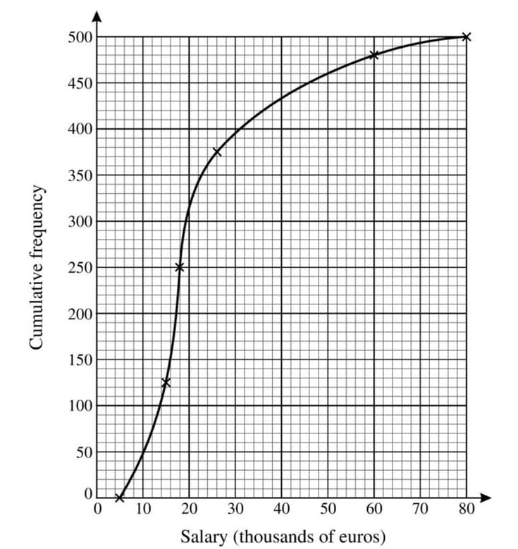
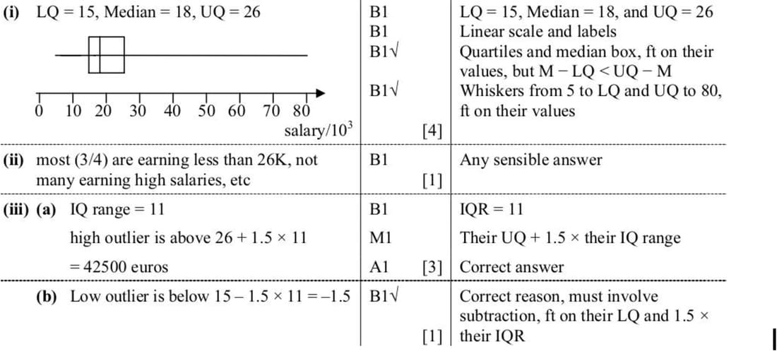
The cumulative frequency graph shows the annual salaries, in thousands of euros, of a random sample of 500 adults with jobs, in France. It has been plotted using grouped data. You may assume that the lowest salary is 5000 euros and the highest salary is 80000 euros.
- On graph paper, draw a box-and-whisker plot to illustrate these salaries.
- Comment on the salaries of the people in this sample.
- An ‘outlier’ is defined as any data value which is more than 1.5 times the interquartile range above the upper quartile, or more than 1.5 times the interquartile range below the lower quartile.
- How high must a salary be in order to be classified as an outlier?
- Show that none of the salaries is low enough to be classified as an outlier.
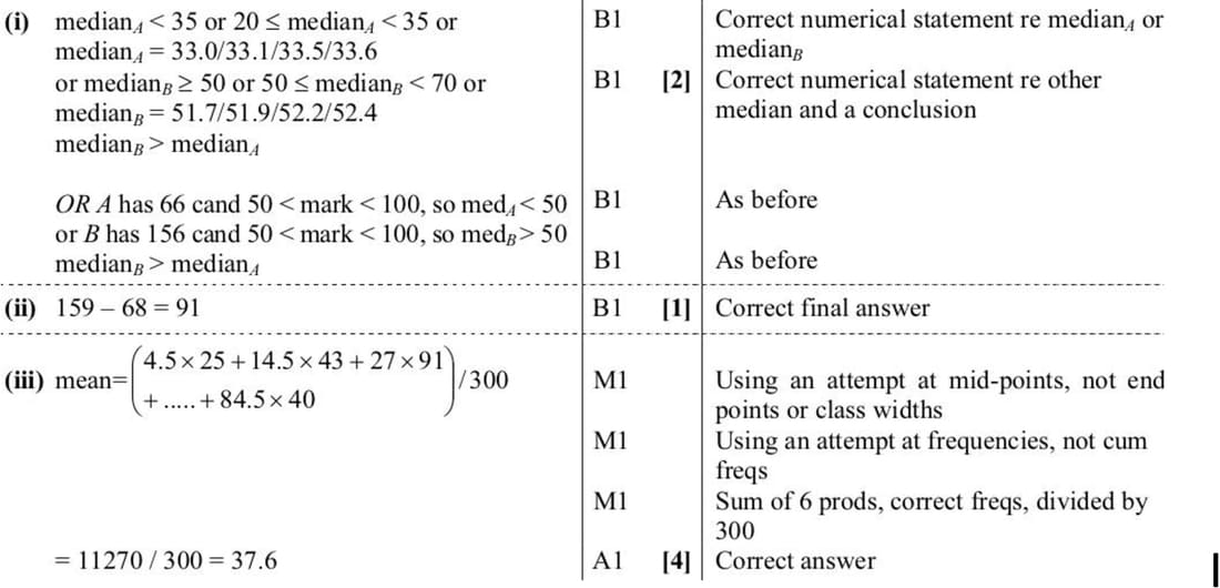
June 2011 p63 q3
The following cumulative frequency table shows the examination marks for 300 candidates in country A and 300 candidates in country B.
| Mark | \(< 10\) | \(< 20\) | \(< 35\) | \(< 50\) | \(< 70\) | \(< 100\) |
|---|---|---|---|---|---|---|
| Cumulative frequency, A | 25 | 68 | 159 | 234 | 260 | 300 |
| Cumulative frequency, B | 10 | 46 | 72 | 144 | 198 | 300 |
- Without drawing a graph, show that the median for country B is higher than the median for country A.
- Find the number of candidates in country A who scored between 20 and 34 marks inclusive.
- Calculate an estimate of the mean mark for candidates in country A.