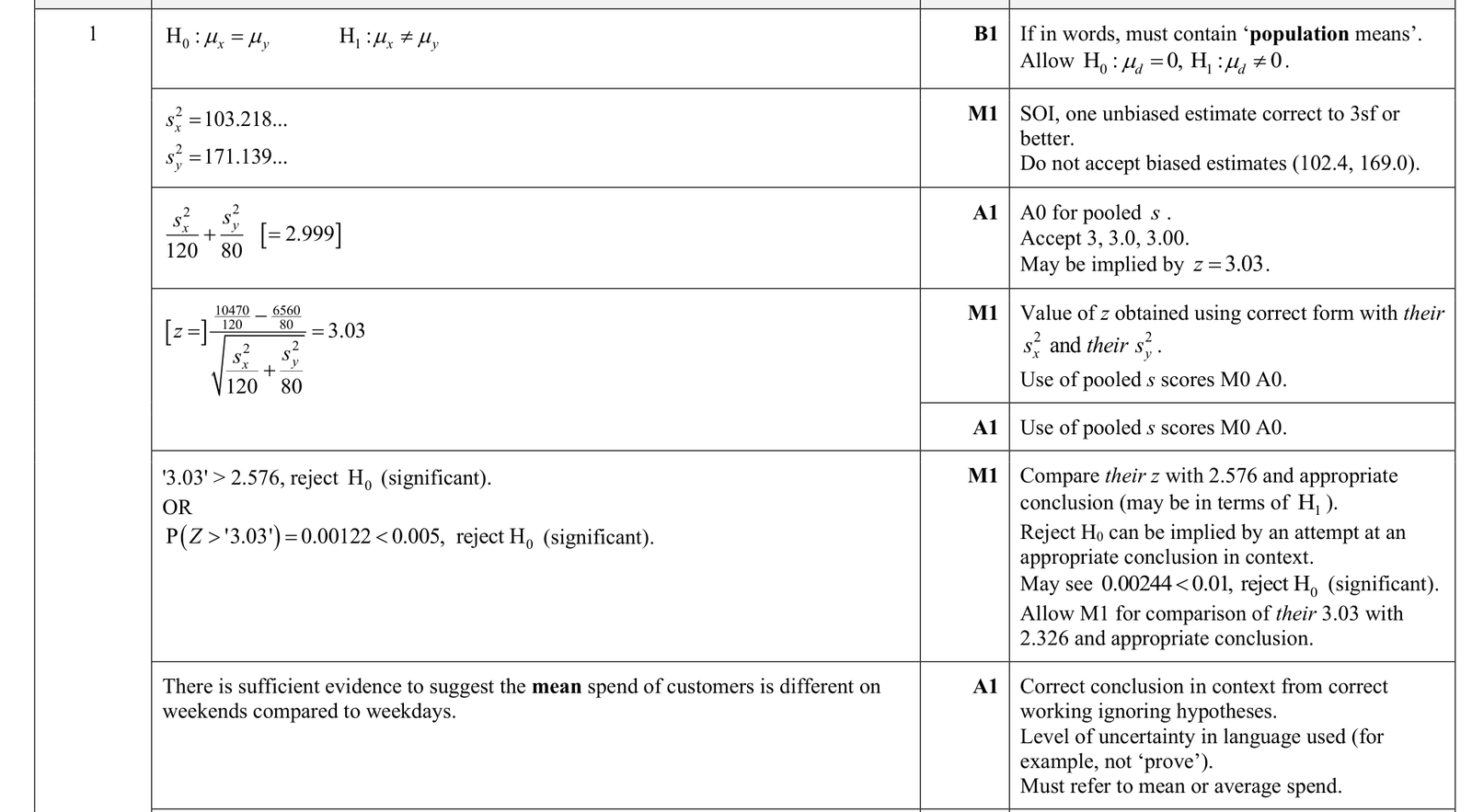
Answer: Let the population mean amount spent on weekdays be \(\mu_x\) and on weekends be \(\mu_y\).

We test

\(H_0: \mu_x = \mu_y\)

\(H_1: \mu_x \ne \mu_y\)

Sample means:

\(\bar{x}=\frac{10470}{120}=87.25\), \(\bar{y}=\frac{6560}{80}=82\)

Unbiased sample variances:

\(s_x^2=\frac{12283}{119}\approx 103.22\), \(s_y^2=\frac{13520}{79}\approx 171.14\)

Since equal population variances are not assumed, use

\(z=\frac{\bar{x}-\bar{y}}{\sqrt{\frac{s_x^2}{120}+\frac{s_y^2}{80}}}\)

So

\(z=\frac{87.25-82}{\sqrt{\frac{103.22}{120}+\frac{171.14}{80}}}\approx \frac{5.25}{\sqrt{2.999}}\approx 3.03\)

For a two-tailed test at the \(1\%\) level, the critical value is \(2.576\).

Since \(3.03 \gt 2.576\), reject \(H_0\).

There is sufficient evidence at the \(1\%\) level to conclude that the mean amount spent per customer is different on weekdays and weekends.

We are comparing two population means, and we are told not to assume the population variances are equal.

So we use a two-sample large-sample test with separate variance estimates.

Let

• \(\mu_x\) = population mean amount spent on weekdays
• \(\mu_y\) = population mean amount spent on weekends

The hypotheses are

\(H_0: \mu_x = \mu_y\)

\(H_1: \mu_x \ne \mu_y\)

This is a two-tailed test.

First find the sample means:

\(\bar{x}=\frac{\sum x}{120}=\frac{10470}{120}=87.25\)

\(\bar{y}=\frac{\sum y}{80}=\frac{6560}{80}=82\)

Now find the unbiased sample variances. Since \(\sum (x-\bar{x})^2\) and \(\sum (y-\bar{y})^2\) are given,

\(s_x^2=\frac{12283}{120-1}=\frac{12283}{119}\approx 103.218\)

\(s_y^2=\frac{13520}{80-1}=\frac{13520}{79}\approx 171.139\)

The standard error of \(\bar{x}-\bar{y}\) is

\(\sqrt{\frac{s_x^2}{120}+\frac{s_y^2}{80}}\)

So

\(\frac{s_x^2}{120}+\frac{s_y^2}{80}\approx \frac{103.218}{120}+\frac{171.139}{80}\approx 0.860+2.139=2.999\)

Hence the test statistic is

\(z=\frac{\bar{x}-\bar{y}}{\sqrt{\frac{s_x^2}{120}+\frac{s_y^2}{80}}}\)

\(z=\frac{87.25-82}{\sqrt{2.999}}\approx \frac{5.25}{1.732}\approx 3.03\)

At the \(1\%\) significance level for a two-tailed test, the critical values are \(\pm 2.576\).

Since \(3.03 \gt 2.576\), the test statistic lies in the critical region, so we reject \(H_0\).

Therefore there is sufficient evidence to suggest that the population mean amount spent per customer is different on weekdays and weekends.

Since \(\bar{x}=87.25\) and \(\bar{y}=82\), the sample suggests weekday spending is higher, although the formal conclusion required is simply that the means differ.